Take the Fourier transform convention , with inverse factor . Then , classically when the boundary terms vanish or in the sense of tempered distributions.
Multiply the given frequency relation by its denominator and then by :Recognizing the four derivative multipliers givesThe convention is stated explicitly because reversing the Fourier exponential changes intermediate frequency signs. The distributional form will matter at the jump of in part (b).
The inverse Fourier transform isFor , close in the upper half-plane, where decays. The single enclosed pole has residue , so counterclockwise integration gives . For , close clockwise in the lower half-plane; there is no enclosed pole and the result is zero. ThusHere is the Heaviside step function. At the jump, symmetric Fourier inversion gives , the average of the one-sided limits. The transform itself cannot fix a function’s value at a single point, so this is the conventional representative rather than extra frequency information.
Factor the cubic denominator as . Substitution givesThere is a double pole at and simple poles at . For , close the inverse-transform contour counterclockwise in the upper half-plane. The residue at the double pole isand the residue at is . Multiplication by from the residue theorem therefore gives .
For , the clockwise lower closure encloses only , with residue . The orientation supplies , giving . Hence the continuous solution isThe large inverse-transform arcs vanish: the rational factor is , while the exponential is bounded on the appropriate closure.
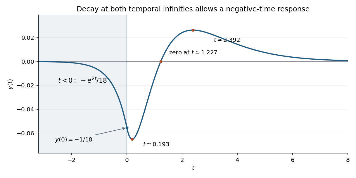
The two-sided decaying Fourier solution; it and its first derivative are continuous at zero
. Details. 
The graph tends to zero from below as , passes through with slope , reaches a small negative minimum after zero, then crosses the axis, reaches a positive maximum and tends to zero from above. The positive-time stationary points solve , and the crossing solves ; these equations determine the sketch without guessing signs.
For a distributional check, and are continuous, while . The jump conditions for a third-order Green function therefore produce the delta in , and each smooth branch satisfies the remaining equation. The nonzero solution for is consistent with the stipulated decay at both temporal infinities. Those are two-sided conditions, not a causality assumption: this is the setting of a decaying two-sided Green function of a constant-coefficient ordinary differential equation and causality versus stability of a Green function.
Articles by others on the same topic
There are currently no matching articles.