Use the ordinary real inner product on the domain of functions obeying the two separated boundary conditions. Integration by parts gives the Lagrange identity for a Sturm-Liouville operatorAt , the two boundary-value vectors and satisfy the same homogeneous linear relation. If , both function values vanish; if , their derivatives are the same constant multiple of their values. Either way . The same argument applies at . HenceThis proves symmetry, and the regular separated Sturm-Liouville problem has the same adjoint domain, so is self-adjoint. To see the domain point, require the boundary form to vanish against every admissible : the independently variable endpoint data force an adjoint-domain function to obey those same endpoint relations.
As usual, each endpoint pair and must be nonzero, and the coefficients must have the regularity needed for these operations. An identically zero pair would impose no condition at that endpoint and would not give the claimed self-adjoint operator. The related operator is self-adjoint in the weighted inner product .
Multiply the eigenvalue equation of the Sturm-Liouville problem by and integrate. Integration by parts givesSince is a nonzero eigenfunction and , the denominator is strictly positive. Thus the Rayleigh quotient isThe endpoint term must be retained for a general Robin boundary condition; it vanishes for homogeneous Dirichlet boundary conditions but need not vanish in the present general problem.
The left boundary condition is , while the right one is . Hence . The Rayleigh quotient becomesEvery term on the right is nonnegative. If the whole expression were zero, in particular , so would be constant. Its zero value at the left endpoint would force , contrary to its being an eigenfunction. ThereforeThis is the positivity mechanism for Dirichlet-Robin eigenvalues on a finite interval. The sign of the boundary contribution is positive for the convention with .
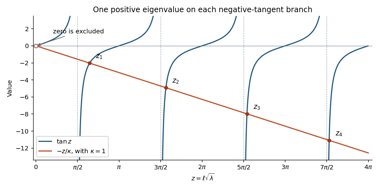
By part (c), write with . The equation is , and the left Dirichlet boundary condition eliminates the cosine term. Thus , with . The right Robin boundary condition becomesPut and . A root cannot have , so this is equivalent to .
On each interval , , the function rises from to a positive value and has derivative . The intermediate value theorem and strict monotonicity therefore give exactly one root there. On the intervening positive-tangent intervals both terms are positive, so there are no further positive roots. ConsequentlyThese intervals establish and an infinite sequence of eigenvalues. The apparent algebraic root of the sine equation is excluded: it gives a zero sine function, and the direct zero-eigenvalue solution would require .

For vector normalization to unit norm, the Dirichlet-Robin eigenvalues on a finite interval giveThe eigenfunctions can otherwise be scaled by any nonzero real constant.
For fixed and , the line becomes increasingly negative, so each intersection approaches its branch’s left-hand vertical asymptote. Write , where and . The eigenvalue equation givesSince , it follows that . ThusThe half-integer phase identifies the sharper high-frequency behaviour of these Dirichlet-Robin eigenvalues on a finite interval. The expansion holds with the Robin coefficient fixed; it is not a uniform expansion in .
For separation of variables, let . The Laplace equation givesA nonzero -periodic angular solution requires , . For , is a linear combination of and , while gives hyperbolic sine and cosine. For , periodicity makes constant, and . Negative separation constants would give nonperiodic real exponentials in .
Superposition yieldsCompleteness follows by expanding a harmonic function in a Fourier series in the periodic coordinate: its Fourier coefficients must satisfy exactly these radial equations. As usual, the coefficients are restricted by the convergence required of the series on compact subregions. The bipolar coordinates domain imposes no boundary condition at or , so both hyperbolic branches remain available.
The only nonzero angular Fourier mode is . Its radial equation is . A solution vanishing at is proportional to ; making its value one at fixes the constant. The Dirichlet problem between bipolar coordinate circles therefore givesIts second derivatives in and cancel, and the endpoint values are respectively zero and . The difference of any two solutions would be a harmonic function with zero Dirichlet boundary conditions, so the maximum principle proves uniqueness.
Geometric wording. In the printed bipolar coordinates, the circle radius decreases with . For , the circle is contained inside the circle. Thus the source’s “inner” and “outer” labels are interchanged geometrically. The solution above follows the explicit coordinate boundary values, which unambiguously specify the problem.
Apply the product rule to the vector field :The two mixed dot products cancel. The divergence theorem, using the outward unit normal, then gives Green's second identity:The usual assumptions are a sufficiently regular boundary and fields with the derivatives and integrability needed for the theorem; singular sources can instead be treated by excising small balls or using distributions.
Define the candidate potential by convolving the decaying Green function with the source. Acting with the Laplacian in the observation variable gives, in the sense of distributions,The final equality is the sifting property of the Dirac delta. The kernel found in part (ii) is locally integrable, and its convolution with a sufficiently regular rapidly decaying source also vanishes at spatial infinity. Thus it satisfies the Poisson equation and the required condition at infinity.
The difference from any other regular decaying solution is a harmonic function on all of space vanishing at infinity, hence is zero by the maximum principle. ThereforeOne can also obtain this expression from Green's second identity on larger and larger balls, with the singularity of the kernel treated distributionally. The surface term at infinity vanishes for the usual potential decay and gradient decay.
Translation and rotation invariance allow a radial Green function , with . Outside the source, , so . Decay at infinity gives .
Integrate the defining equation over a small ball centred on the source. The divergence theorem fixes its flux:ConsequentlyThis is the Green function of the Laplacian with the stated negative-delta sign. A homogeneous addition would change the delta normalization, so the singular coefficient is fixed, not an arbitrary integration constant.
Write , . For a spherical source, the angular integral needed for the Green function of the Laplacian isThis is the angular form of the spherical shell theorem. Substituting the source into the Green function integral therefore yieldsThe elementary integrals areThe terms proportional to cancel, leavingThe value at the origin is the continuous limit. At large radius , consistent with the integrated source and the factor in the far-field potential.
For a direct check, set . Then , so for . Boundedness of at zero cancels the singular terms and excludes an extra point source. The original density is itself singular but locally integrable; the equation at the origin is understood in the sense of distributions. This is the Poisson potential of an exponential-over-radius source with amplitude .
Choose , so on the arc. Its clockwise orientation givesBecause is an analytic function at zero, uniformly on the small arc. Integration then givesThereforeThe estimation lemma also gives . Hence a sufficient large-arc condition isFor example uniformly on the arc, with , suffices. Under the stronger literal assumption that is analytic at infinity, its Laurent expansion is ; the necessary and sufficient condition is then . A nonzero constant term would instead give the growing contribution .
For , the upper-bank argument tends to zero, whereas the lower-bank argument tends to . ThusThe analytic function has identical boundary values across this part of the real axis. Hence the branch cut introduces a sign change:This compares integrand values. When two contour segments traverse opposite banks in opposite directions, their orientation supplies an additional minus sign.
The rational factors give four simple poles at ; none is canceled by the numerator. The square root has branch points at , with local behaviour proportional to in the integrand.
For this part, choose analytic off and satisfying at infinity. Its values are for , for , andThus the chosen branch cut is , and the function is analytic elsewhere apart from the four poles. Infinity is not an intrinsic branch point: on this branch.
Another legitimate convention applies the positive-axis square root of part (a) to ; it places the cuts on and . Its upper-half-plane values agree with the branch used here, so the contour calculation below and the positive real square root in the required integral are unchanged. The branch choice must be stated because a square root alone does not specify a single-valued complex function.
Use the branch from part (i) and close the real-axis path with a large upper semicircle, indenting clockwise around and . On the segment between them, take the upper-bank value of the branch cut. This is an instance of square-root endpoint integrals by an upper-half-plane contour.
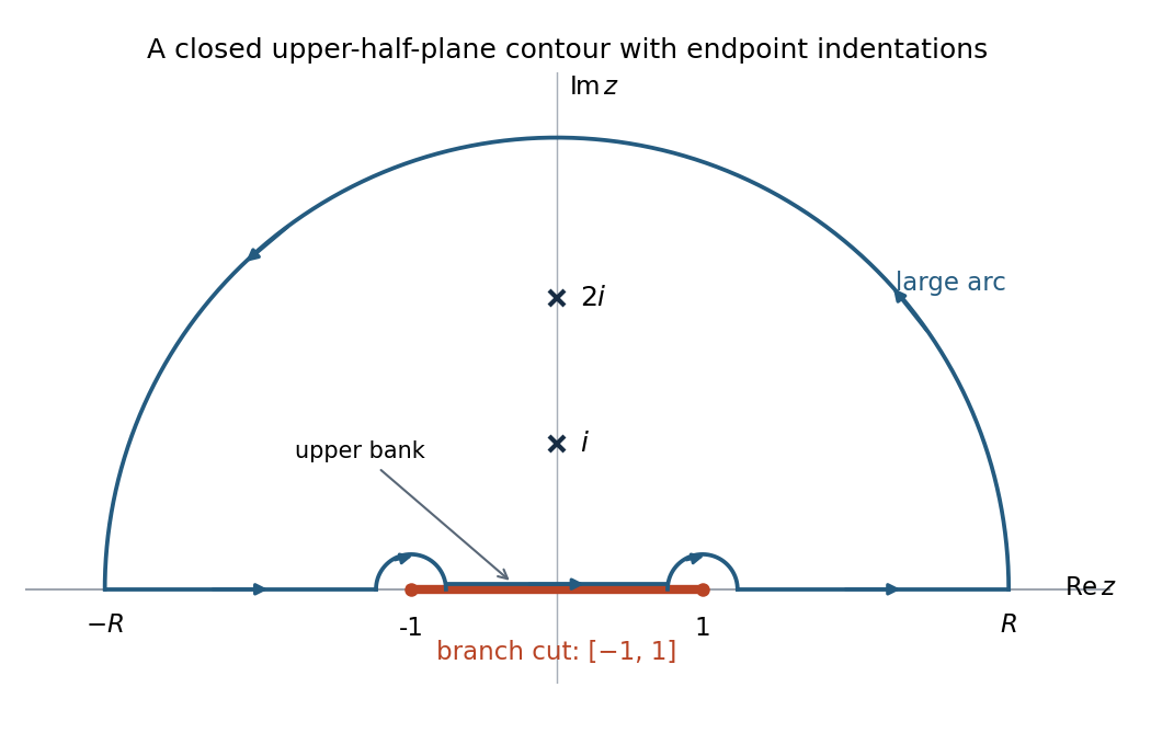
Upper-half-plane contour, clockwise endpoint indentations, and the two enclosed poles; indentation sizes are exaggerated
. Details. 
The contributions can be controlled separately. Since , the large arc contributes . Near either branch point, , so an arc of length contributes . On the upper bank of ,which is odd in , so its integral is zero. On the exterior real intervals , while the rational numerator is odd. Hence and the two exterior contributions sum to .
The enclosed residues use and :The residue theorem gives . ThereforeAs an independent check, converts the integral towhich yields the same value. This check also confirms the branch signs and the factor of two in the contour argument.
Take the Fourier transform convention , with inverse factor . Then , classically when the boundary terms vanish or in the sense of tempered distributions.
Multiply the given frequency relation by its denominator and then by :Recognizing the four derivative multipliers givesThe convention is stated explicitly because reversing the Fourier exponential changes intermediate frequency signs. The distributional form will matter at the jump of in part (b).
The inverse Fourier transform isFor , close in the upper half-plane, where decays. The single enclosed pole has residue , so counterclockwise integration gives . For , close clockwise in the lower half-plane; there is no enclosed pole and the result is zero. ThusHere is the Heaviside step function. At the jump, symmetric Fourier inversion gives , the average of the one-sided limits. The transform itself cannot fix a function’s value at a single point, so this is the conventional representative rather than extra frequency information.
Factor the cubic denominator as . Substitution givesThere is a double pole at and simple poles at . For , close the inverse-transform contour counterclockwise in the upper half-plane. The residue at the double pole isand the residue at is . Multiplication by from the residue theorem therefore gives .
For , the clockwise lower closure encloses only , with residue . The orientation supplies , giving . Hence the continuous solution isThe large inverse-transform arcs vanish: the rational factor is , while the exponential is bounded on the appropriate closure.
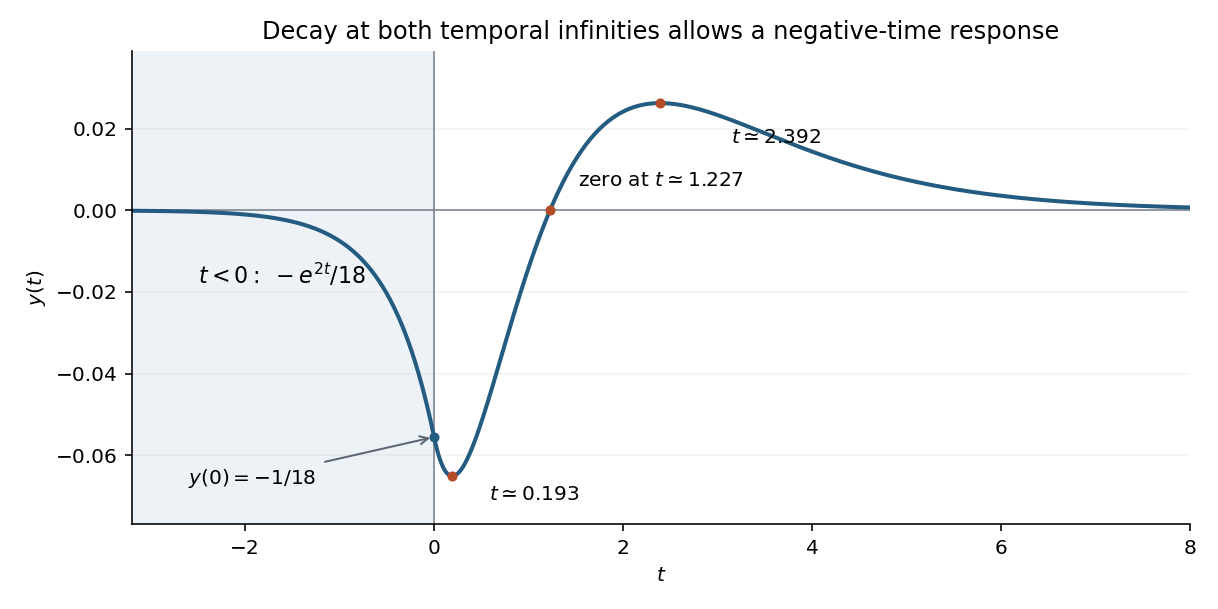
The two-sided decaying Fourier solution; it and its first derivative are continuous at zero
. Details. 
The graph tends to zero from below as , passes through with slope , reaches a small negative minimum after zero, then crosses the axis, reaches a positive maximum and tends to zero from above. The positive-time stationary points solve , and the crossing solves ; these equations determine the sketch without guessing signs.
For a distributional check, and are continuous, while . The jump conditions for a third-order Green function therefore produce the delta in , and each smooth branch satisfies the remaining equation. The nonzero solution for is consistent with the stipulated decay at both temporal infinities. Those are two-sided conditions, not a causality assumption: this is the setting of a decaying two-sided Green function of a constant-coefficient ordinary differential equation and causality versus stability of a Green function.
A second-order Cartesian tensor assigns components in each orthonormal coordinate system according toHere is the matrix taking old vector components to new ones, and repeated indices are summed. This is the tensor component transformation law; an arbitrary array of nine numbers is not a tensor unless its components in different frames obey this rule. No symmetry is implied by being a second-order tensor.
Let be an orthogonal change of axes. Since is a second-order tensor, . The scalar-contraction assumption givesfor every tensor . In one fixed frame its components can be any array: in particular, choose one component at a time to be one, all others zero. Equality of the coefficients then forcesMultiplying by and yieldsThis is exactly the tensor component transformation law. It is the full-contraction version of the quotient theorem for Cartesian tensors. The words “for every” are essential: testing a single , such as the zero tensor or the identity, would not determine all components.
Use the quarter-turn rotation matrixFor a general second-order tensor, direct multiplication givesRequiring gives , , together with , and together with . Thus all mixed axial-transverse entries vanish andFor an arbitrary rotation angle , the transverse rotation is , where . The transverse block of is , so it commutes with . Therefore , while the axial component is unchanged.
Hence invariance holds under every rotation about the axis, not just the quarter-turn. This is the general axisymmetric second-order tensor; a symmetric tensor would additionally require , but that restriction was not assumed.
For , the inertia tensor component is . Reflect either coordinate appearing once: the cylindrical domain and density are unchanged, while the integrand changes sign. Thus every off-diagonal component vanishes. Rotational symmetry also implies .
Use cylindrical coordinates , , , with volume element . The axial moment of inertia isThe two contributions to a transverse component areThereforeThe axial value and transverse value for , give an independent check on both diagonal entries.
For a zero-natural-length spring, extension is the full distance between its endpoints, so the squared spring lengths are quadratic functions of the Cartesian coordinates. The Lagrangian isThe gravitational potential energy has positive derivative in the upward coordinate, giving downward forces. Applying the Euler-Lagrange equations to all four coordinates givesThe two spring forces are equal and opposite on the two masses for the connecting spring, as required by Newton's third law.
At equilibrium, the two horizontal equations imply and then , so both vanish. Adding the two vertical equations gives ; the second separately gives . HenceRetain the imposed constraint and set , , . Subtracting the equilibrium equations cancels all constant gravitational terms. For , the small-oscillation mass and stiffness matrices areThe horizontal reaction enforcing the constraint replaces the removed equation; it is not necessary to demand that the original unconstrained horizontal force on mass 2 vanish during motion. Because the zero-natural-length spring potentials are exactly quadratic, these displacement equations are actually exact within the ideal spring model, not merely first-order approximations.
Keep the constraint from part (b). For equal masses and spring constants, the generalized eigenvalue problem for small oscillations reduces toThe horizontal coordinate decouples, givingIn this normal mode, mass 1 oscillates horizontally, mass 2 has its horizontal coordinate fixed, and neither mass has a vertical displacement.
For the vertical block, write . Its characteristic polynomial is . Thus , and the first vertical equation gives . If is the golden ratio, the two vertical modes areIn the lower-frequency mode, the masses move vertically in phase, with the lower mass having the larger amplitude. In the higher-frequency mode they move oppositely, with lower-to-upper amplitude ratio . Their Euclidean inner product is zero because ; since , this is also mass-matrix orthogonality of normal modes.
The three frequencies satisfy . Each mode has a scalar coordinate , and their superposition gives the general constrained motion. No zero-frequency mode remains because the first spring anchors the system. Gravity fixes the equilibrium extensions but drops out of these frequencies for zero-natural-length springs.
The quotient group consists of the cosets , with multiplicationFor well-definedness, replacing representatives by and changes their product to . Since is a normal subgroup, the final two factors lie in , so the product coset does not change.
Associativity follows from that in ; the identity element is the coset , and . Hence these cosets form a group. By Lagrange's theorem, every subgroup has order dividing , and its subgroup index is . In particularNormality is needed for the quotient multiplication, whereas Lagrange’s counting formula holds for every subgroup.
The four displayed matrices fail closure: for example is not one of them. Thus they do not form a group by themselves.
Let and . The enlarged set is the single-qubit Pauli groupThere are 16 distinct matrices: are linearly independent, so two different ones cannot be scalar multiples, and the four phases are distinct for each nonzero matrix.
The Pauli matrices satisfyHere is the Kronecker delta and the Levi-Civita symbol. Thus any product of two Pauli matrices is another Pauli matrix or the identity times a phase in . Multiplying by the two original phases preserves membership in , proving closure of all 16 matrices.
Associativity is inherited from matrix multiplication, the identity is , andThis proves every group axiom. The resulting group is non-Abelian, since reversing changes its sign.
For every positive integer , the group laws give . ConsequentlyThe sets of positive exponents returning the two elements to the identity element are identical. If this set is nonempty, its least member is the order of a group element in both cases. If it is empty, neither element has finite order. Therefore, including the infinite-order case,For a direct divisibility argument in the finite case, if has order , then , so its inverse’s order divides . Reversing the roles shows divides that order, forcing equality. This is the general fact that an element and its inverse have the same order; it also reflects as cyclic subgroups.
Write with . For any , the normal subgroup property implies . This conjugate cannot be , since multiplication by and would then give . There is only one remaining choice, soThus commutes with every element of ; the identity does too. HenceThis proves that a normal subgroup of order two is central. The proof does not require to be finite: conjugation permutes and fixes its identity, so it must fix its only other element.
A group homomorphism is a map preserving multiplication:It necessarily sends to and sends inverses to inverses, by applying this relation to and . Its kernel of a group homomorphism isThe kernel is a normal subgroup of the domain: if and , then . The kernel’s identity condition refers to the identity in the target group.
Let be a proper subgroup. By Lagrange's theorem, divides . Since , its possibilities areThe subgroup of order one is generated by the identity and is cyclic. For either prime order or , choose other than the identity. Its order of a group element divides and is not one, so it is . Thus its powers exhaust , proving .
ThereforeThis uses the fact that a group of prime order is cyclic. It does not require the order-21 group itself to be Abelian or cyclic.
Since , a representation satisfies . Orthogonality gives , while the involution relation gives . Hence is a symmetric matrix, so .
Its entries obeyIf , then ; putting and gives a reflection. If , the diagonal entries are independently : the opposite-sign cases are already included among these reflections, while equal signs give or . Faithfulness excludes , since . Therefore the orthogonal involutions of the plane giveThe first is rotation by . The second is reflection in the line making angle with the first axis: the unit vector along that line is fixed, and its perpendicular is negated. These are all the nonidentity orthogonal transformations of order two in the plane.
A cyclic group of order contains an element of order two if and only if divides . Necessity follows from Lagrange's theorem; for even , the unique such element is . HenceBecause has order and the representation is faithful, cannot be a reflection, which has order two. It is therefore a rotation through a primitive angle , with . The condition on the greatest common divisor is exactly what makes its order rather than a proper divisor. Since is even, is odd, so is the half-turn:The character is the trace:Choosing the primitive generator with gives the customary rotation representation. The general coprime value is included because faithfulness alone does not select that generator. These are the two-dimensional cases in the irreducible real representations of a finite cyclic group.
Write . The matrix is a reflection by part (a). Reflection reverses a rotation angle, giving . Faithfulness lifts this matrix identity back to the group:Moving each past a rotation reduces every word to or , . These elements are distinct: the rotations are distinct by the order of , and reflections have determinant , so cannot equal a rotation. ThereforeHere the subscript denotes group order. This is the reflection case of finite subgroups of the plane orthogonal group.
Every has square , so there are reflection subgroups of order two. Within the rotations, the even- assumption from part (b) supplies the additional half-turn . Distinct involutions generate distinct two-element subgroups. ThusFor comparison, without the evenness requirement the corresponding odd- count would be . The even case agrees with involutions in an even dihedral group.
For , takeDirect multiplication gives , so . The product rules arewith exponents modulo four. They yield the complete multiplication table, where the row element multiplies the column element on the left:This is the symmetry group of a square, the dihedral group of order eight, often written when its subscript counts vertices instead. Its five order-two subgroups are generated by .
Articles by others on the same topic
There are currently no matching articles.