At a vertex with exterior turning angle , the interior angle is . A local conformal map from a half-plane therefore behaves as , so its derivative has local exponent .
On each real boundary interval between prevertices, is constant because the image is a straight side. Across a prevertex its change is the exterior turning angle. Taking , the product has exactly these changes. Dividing by that product removes the corner singularities and leaves a holomorphic nonzero function with constant boundary argument. Schwarz reflection and the regular behavior at infinity make it constant. This gives the Schwarz-Christoffel formulaThere are three freely normalizable real prevertices, because an automorphism of the upper half-plane has three real parameters. After those are fixed, the remaining prevertex parameters are determined by the polygon's shape through the side-length conditions. They are not further independent normalization choices.
If the last prevertex is at infinity, absorb its constant scale into and omit its finite factor:For a bounded polygon, , so this derivative behaves like , consistent with the corner described in the local coordinate .
Use the branch of that is positive for , . The right-half-plane slit mapis holomorphic in the upper half-plane, with derivative , the required Schwarz-Christoffel formula form. Its derivative has no interior zero.
To verify the image and global injectivity, factor the construction. Squaring maps the upper half-plane bijectively onto . Thus ranges over . The positive-real-part square root maps this onto the right half-plane with the interval removed; reciprocation maps it onto the right half-plane slit along . This also identifies the slit tip as a boundary point; the strict inequality in the printed slit description must be understood with that boundary convention.
Approaching the real axis from above givesIn particular maps to the lower infinite prime end , to the tip , and to the upper infinite prime end . The real-axis point at infinity maps to zero on the vertical wall.
Let , so , choosing the analytic branch with ; for example . Let be the source point. For the convention , the Dirichlet Green function in the upper half-plane is obtained by an opposite-sign reflected source:It vanishes for real , has the logarithmic singularity , and is harmonic elsewhere. Conformal invariance of two-dimensional harmonic functions now givesThe branch specified above maps every boundary bank to the real axis, so the Green function vanishes on both slit banks and the vertical wall. Local conformality preserves the coefficient of the logarithmic singularity. If the convention is instead , negate this expression.
Orient the smooth contour so the plus side is to its left. Assume the density is Hölder continuous near the observation point and the integrals converge at any other endpoints. The Cauchy principal value isSubtract from the numerator. The resulting quotient is locally integrable, so its limits from the two sides coincide. For the remaining constant density, straightening the contour gives a half-circle contribution . Division by yields the Sokhotski–Plemelj formulaFor the requested real integral assume and , ensuring integrable endpoints and an interior principal-value pole. Put . Choose analytic off , positive for , and at infinity. Its two boundary values are .
The jump is . The Cauchy representation for this decaying analytic function is therefore . Taking the mean of its two boundary values removes the half-residue terms and gives
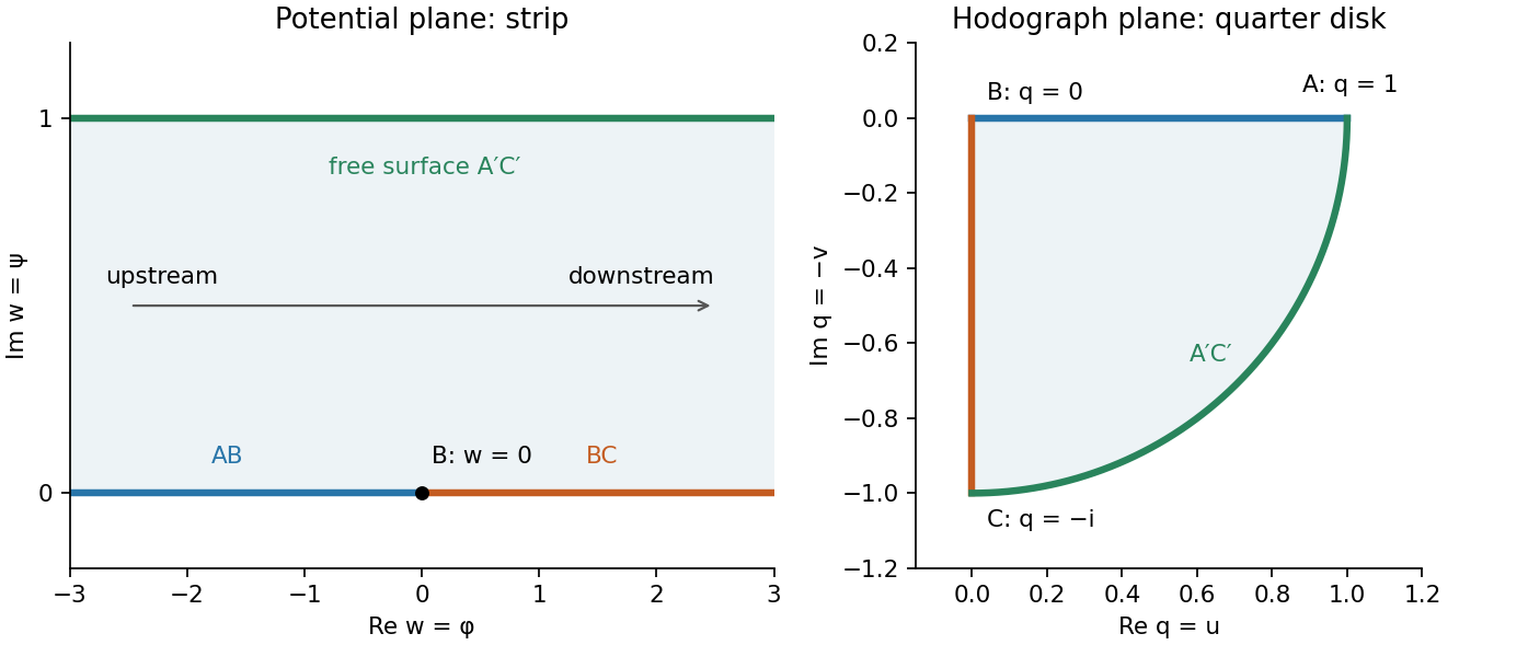
The complex potential of a two-dimensional potential flow maps the fluid region to the strip . Its lower boundary is the wall, with at ; upstream is and downstream is . The free streamline is the upper strip boundary.
Write . The horizontal wall gives positive real velocities running from to the stagnation value at . The vertical wall gives negative imaginary velocities from zero to . On the free surface , with the angle turning continuously from zero to . Thus the hodograph plane domain is the fourth-quadrant quarter of the unit disk, bounded by those two radii and the unit-circle arc.
The following successive conformal maps straighten it. First maps to the lower half unit disk. Next maps to the third quadrant, since and . Finally maps onto the upper half-plane. The three wall landmarks go to respectively.
The strip map also maps onto the upper half-plane, with these same landmarks . The unique half-plane automorphism fixing all three is the identity. ThereforeThe free surface maps to the negative real axis in either construction, as required by its streamfunction value one. This completes the right-angle free-streamline hodograph map construction.

Glue the two analytic functions on their overlap, where their values agree. Since , the two half-planes cover the whole complex plane. The gluing therefore defines an entire function. It is bounded outside a sufficiently large disk by the two given infinity bounds, and bounded on the remaining compact disk by continuity. The Liouville theorem then gives one common constant.
For the standard canonical Wiener-Hopf factorization, first assume the nonzero kernel has Index of a Wiener-Hopf kernel zero and a continuous analytic logarithm tending to zero at both ends of the strip, with sufficient decay for the Cauchy projections. Choose . Let be the line oriented left to right, with its factor used above that line; let be the line oriented left to right, with its factor used below that line.
For , closing the rectangle between the two lines and using the Cauchy integral formula givesThus . Multiplying gives in the overlap. The canonical factors are analytic, nonzero, and normalized at infinity in their respective half-planes, so part (a) yieldsContours may be shifted within the strip without changing their factors on the appropriate side. When necessary, a subtracted Cauchy kernel fixes convergence and the common normalization constant.
The printed hypotheses omit the index and factor-growth qualifications; alone does not ensure them. An explicit counterexample is on , with and . Both functions are analytic and bounded at infinity in their prescribed half-planes, and the relation holds. If admissible analytic factors made their common product a nonzero constant, would force constant and hence proportional to , impossible because has a pole at in the plus half-plane. The natural factors , instead give the nonconstant common polynomial . Thus the boxed constant conclusion is the intended index-zero result, not a consequence of the literal assumptions alone.
Let . On the negative half-line, the integrand magnitude is bounded at infinity by a constant times , which is integrable as when . On the positive half-line the corresponding bound is , integrable when . ThusOn compact subsets strictly inside these half-planes, the same exponential domination absorbs every power of . Differentiation under the integral is therefore valid and proves holomorphy, rather than only absolute convergence. The bars here denote the printed one-sided Fourier transforms, not complex conjugation.
Use the Fourier convention . Transforming the differential equation givesDefine analytic above the downward cut from zero, and analytic below the upward cut from . More explicitly take and . In the strip , put . Then and ; at , , fixing the choice throughout the strip. The decaying mode is .
The positive-half-line boundary value has transform for . Thus and . The transformed boundary relation isLet . Splitting off the pole at zero givesThe left side is analytic in the lower domain up to : its apparent pole at zero is removable. The right side is analytic for . By the supplied boundedness of and , both sides tend to zero at infinity in their half-planes. The gluing and Liouville theorem argument therefore makes their common value zero. ConsequentlyChoose the inversion contour oriented left to right, with any fixed . It passes above the pole at zero and below the branch point at . Fourier inversion gives exactlyThus the appropriate value is . The other proposed value reverses the residue of the boundary step and violates its prescribed positive value.
There is also a far-field qualification in the source. The formula is the intended bounded mixed-boundary solution, but it does not tend to zero along every path to infinity. This can be checked explicitly: in parabolic coordinates , , with , the mixed-boundary convection-diffusion solution in parabolic coordinates isIndeed and ; the identity proves the differential equation. At the boundary value is one, and at its normal derivative is zero. Its traces are for and for , whose one-sided transforms are the expressions derived above.
At a fixed angle away from the positive axis, and . But at fixed and , and . Hence the radial decay statement cannot hold uniformly as printed; the intended decay is away from the downstream boundary layer. The exact expression also identifies its thickness as .
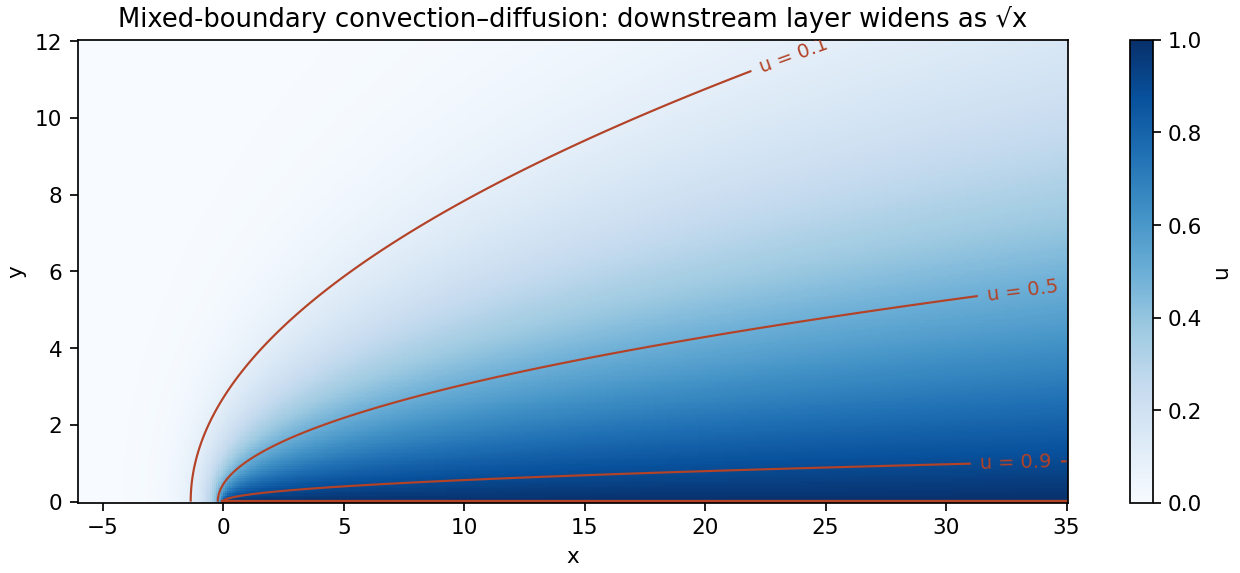
The exact mixed-boundary solution decays away from the downstream boundary layer
. Details. 
Articles by others on the same topic
There are currently no matching articles.