A differential equation is an equation relating an unknown function to its derivatives. It specifies how change depends on the present state, and sometimes on the independent variables themselves. A solution of a differential equation is a function satisfying that relation throughout a stated domain; giving a formula without its domain can conceal a point where the equation is undefined.
The central idea is to turn a local law into a whole trajectory. For example, , with constant , says that the instantaneous derivative is proportional to the current value. If and per day, the solution of a differential equation is , so . This is an ideal growth model assuming a constant proportional rate; the exponential function emerges from repeatedly applying the same local rule. Changing the sign of gives exponential decay.
An ordinary differential equation uses one independent variable. A partial differential equation can involve several, such as space and time, and uses partial derivatives. Additional information selects a particular solution of a differential equation: an initial condition describes a starting state, whereas a boundary condition imposes constraints at the edge of a domain. The useful questions extend beyond finding a formula: does a solution of a differential equation exist, is it unique, and what happens to it over time?
An orthogonal trajectory intersects every regular member of a specified family of plane curves at a right angle. If eliminating the family parameter gives its tangent slope , the dot product of the two tangent directions gives the orthogonal slope wherever both slopes are finite and nonzero. Vertical and horizontal tangent directions are interpreted geometrically. For the family with , eliminating gives , and the orthogonal trajectories satisfy . For these are ellipses; for they are circles.
A stationary solution of an evolution differential equation is independent of time. Substituting leaves the spatial boundary value problem that determines its profile. For an ordinary differential equation this is an equilibrium; for a partial differential equation it may vary in space. A stationary profile need not have zero flux, although zero flux is forced in a one-dimensional conserved system with reflecting endpoints.
A direction field for places a short segment with slope at each sampled point where is defined. A function graph of a solution of a differential equation follows these segments: its tangent line has exactly the prescribed slope. Segment length is a drawing choice, rather than a speed; arrows, if used, point toward increasing . An isocline collects points with one common slope.
For Newton's law of cooling, with time in minutes and temperature in degrees Celsius, the slopes at are respectively degrees Celsius per minute. Each horizontal row is an isocline, because this autonomous differential equation has no explicit time dependence. Above the solutions of a differential equation descend, below they rise, and is an equilibrium point.
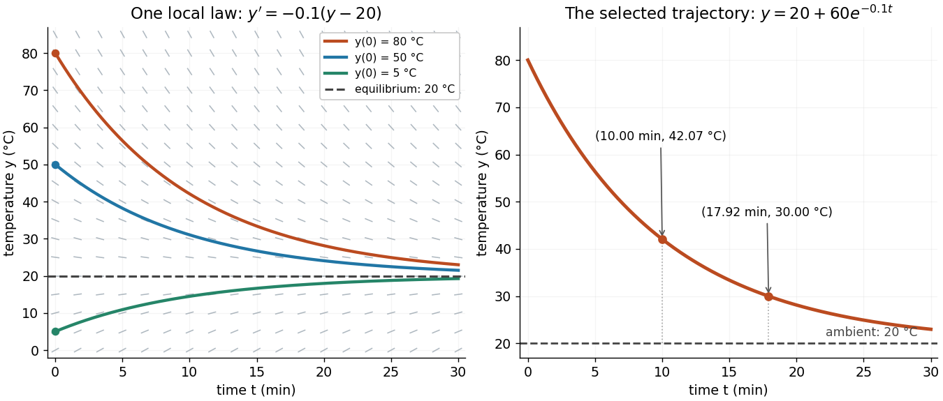
The highlighted initial condition selects one curve from the family. The picture reveals approach to the equilibrium point before any algebra is done. Under the hypotheses of the Picard-Lindelöf theorem, distinct function graphs of solutions cannot cross or even meet in the time-state plane. A direction field alone does not guarantee uniqueness: several curves can share a tangent line at the same point when those hypotheses fail. See the delayed-start example under initial value problem.
This geometric interpretation is developed in Direction Fields, Isoclines, Integral Curves.
For the first-order ordinary differential equation defined on an open subset of the plane, an isocline of slope is the level setHere is a constant. At every point of this isocline, the direction field prescribes a tangent vector proportional to for a solution of a differential equation. It does not generally prescribe the tangent line of the isocline itself. The level set can have several components or fail to be a smooth curve, and points outside are excluded.
For example, take on the whole plane. Its isoclines are the parallel straight linesEach line has slope , while the direction field along it has slope . Thus the isocline carries horizontal segments even though the line itself rises. A function graph of a solution of a differential equation follows the segments, rather than following this line. Only the isocline with , namely , is also a solution of a differential equation.[ref]
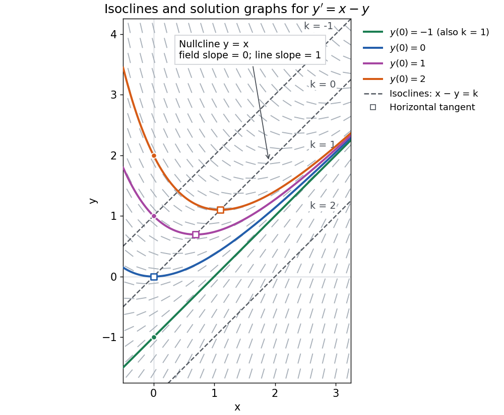
The first-order linear differential equation has the exact familyThe initial condition selects and hence a unique solution of a differential equation for every real . The picture shows . For the solution of a differential equation stays on the isocline; for other it moves through different isoclines. These formulas check the pictured trajectories by direct differentiation, independently of how the direction field was sampled.
The zero-slope isocline is called a nullcline. Below the nullcline in this example, ; above it, . For , the solution of a differential equation meets it at , where and , a strict local minimum. The nullcline is therefore a useful guide to turning points, although it is not itself a solution of a differential equation. In the equivalent planar autonomous differential equation , , it is the nullcline for the second component; there is no equilibrium point, because the first component never vanishes.
This makes isoclines useful even when no explicit solution of a differential equation is available: organize a direction field by common slopes, read where function graphs rise or fall, and identify possible turning points on nullclines.
A jump condition relates the one-sided limits of a solution or its derivatives across a discontinuity or singular forcing. Integrating a differential equation across a shrinking interval containing a Dirac delta source determines the permitted jump. A jump condition for an impulse and Rankine-Hugoniot condition are specific instances with different governing equations.
A delay differential equation relates a derivative at the current argument to values at earlier arguments. For example, the Buchstab function obeys for .
The defining feature is memory: a derivative can depend on earlier values of the unknown function. Constant delays, time-dependent delays, and delays depending on the unknown function belong to this wider class. The retarded delay differential equation below isolates a single positive constant delay.[ref]
Delay-differential equations by Skip Thompson. Skip Thompson, Delay-differential equations, opening definition and equation (1): constant and state-dependent delays
The Malthusian delay differential equation is a simple linear member of this class. The method of steps for a delay differential equation constructs its future from a history function of a delay differential equation, and the characteristic equation of a delay differential equation studies its exponential function modes. The exact polynomial steps for a delay equation below make that construction explicit without approximating the solution of a differential equation. Applications include population dynamics and feedback control; the delayed negative feedback model and feedback delay explain why the timing of a return matters as well as its sign.
For a smooth delayed-transfer epidemic model, the incidence equals . Substituting the zero-delay equations only inside the correction gives . The correction has opposite signs in the receiving and departing compartments, preserving their transfer balance.
For nonnegative instantaneous damping and positive delayed gain , characteristic roots obey . There is no nonnegative real root. The first imaginary crossing has and , . In particular stability is retained below this first boundary and is exact only at . For small positive , the critical gain is and the scaled period tends to four. If the time delay is dimensional , that period is multiplied by .
This delay differential equation replaces instantaneous logistic inhibition by a population value one delay earlier. A positive history function of a delay differential equation gives positive solutions while they exist. The equilibria are zero and one. Linearization at one gives , with characteristic equation . Delayed sign reversal permits overshoots around one and, at the delayed logistic Hopf threshold, a periodic branch.
A purely imaginary root of has frequency one and first appears at . Roots cross with positive real derivative ; all roots lie in the left half-plane for smaller positive delay, since a hypothetical root with would require both and . A small-amplitude expansion yields and , verifying a nondegenerate Hopf bifurcation. The limiting period is .
For a single constant delay , a retarded delay differential equation has the displayed form: delayed values of the unknown function enter, but delayed first derivatives do not. The unknown can also be a vector.[ref]
Delay-differential equations by Skip Thompson. Skip Thompson, Delay-differential equations, opening definition and equation (1): delayed values versus delayed derivatives
Here denotes time, and the rule applies for , with a right derivative at . On , the argument lies in the prescribed past. Once this interval is known, it supplies the delayed values for . This is the method of steps for a delay differential equation: solve successive ordinary differential equations with a known delayed input, keeping each new endpoint as the next initial condition. For a continuous function locally Lipschitz continuous in its two state arguments, locally uniformly in , this gives local existence and uniqueness for each continuous history function of a delay differential equation, while the solution of a differential equation remains in the domain of . A nonlinear rule can still produce finite-time blowup.
A history function of a delay differential equation supplies the past interval needed to start a retarded delay differential equation. A single initial condition generally leaves earlier delayed values unspecified.[ref]
Delay-differential equations by Skip Thompson. Skip Thompson, Delay-differential equations, Initial History Function: prescribing the solution before the starting time
For a continuous function history, the natural state at time is the entire segmentIt belongs to the function space , an infinite-dimensional vector space: the functions are linearly independent. Shifting forward retains the part of the past that the equation can still read. Thus even one scalar unknown can require a state in an infinite-dimensional vector space.
The insufficiency of one value is visible without any approximation. Consider with the two history functions of a delay differential equationBoth give , yet on the first step the respective derivatives are and . Direct integration givesIn particular while . On the next step,At they are and , a gap of . These different futures reflect different prescribed histories; each fully specified problem has a unique solution of a differential equation. More strongly, for with , observing the entire first-step derivative recovers every history value through for , using the right derivative at . The future can depend on the whole function, rather than a finite list of its samples.
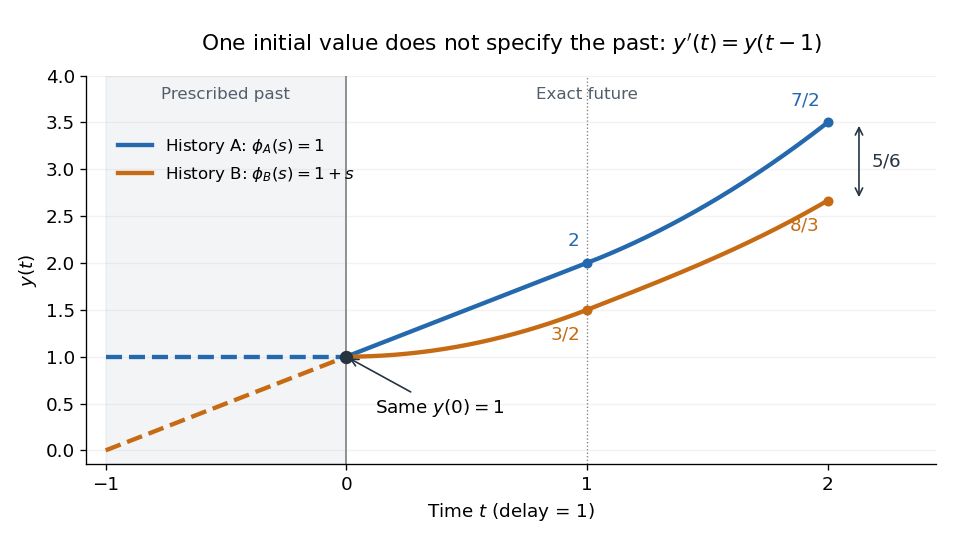
Equal initial values and different histories give different futures
. Two exact solutions of a differential equation for . Dashed curves are the prescribed history functions of a delay differential equation; solid curves are their exact continuations. Both pass through . The endpoint values and come from the displayed polynomials, with no numerical time stepping. Details.Use the Malthusian delay differential equation with time measured in units of its constant delay:Here is a real constant. On the first interval , hence . On the next interval the delayed input is , already known, so the method of steps for a delay differential equation givesEach polynomial integrates the preceding interval's delayed polynomial, and its integration constant ensures continuity. At , the step endpoints are , , and . At , the value is , but its derivative is the earlier value . This is the geometric distinction from the ordinary differential equation , whose derivative would equal its current value.
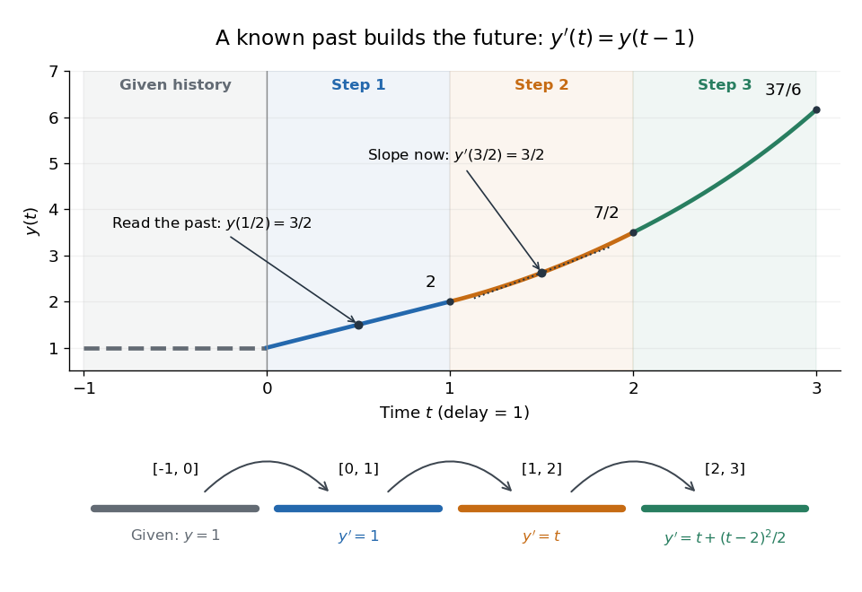
A prescribed past becomes successive exact polynomial steps
. The history function of a delay differential equation is and . Each colored interval supplies the delayed input for the next one; the lower panel gives that next interval's derivative. The marked tangent line at has slope . All curves are evaluated from exact polynomials. Details.More generally, for any integer ,At an integer join the newly introduced term vanishes. Inside a step, differentiation lowers each power by one and gives exactly times the preceding step evaluated at . Together with , this verifies the formula by mathematical induction; it is an exact construction, not a truncated power series.
The history and the new equation need not prescribe matching derivatives at the starting time; their mismatch can reappear later in higher derivatives.[ref]
Delay-differential equations by Skip Thompson. Skip Thompson, Delay-differential equations, Derivative Discontinuities: initial incompatibility and its propagation
In this example, and . For , is continuous at but jumps there by ; at , the first jump is in , of size . The solution of a differential equation is therefore continuously differentiable for positive time, although it need not have continuous derivatives of every order at step boundaries.A classical solution is a sufficiently differentiable function that satisfies a differential equation and any prescribed initial or boundary conditions. A weak solution instead satisfies an appropriate integral or distributional identity in a specified function space. For a smooth locally Lipschitz continuous vector field, an ordinary differential equation has a unique local solution for each initial state; this does not by itself ensure global existence or boundedness.
An ordinary differential equation relates an unknown function of one independent variable to its ordinary derivatives. Its order is the highest derivative appearing. Thus is first order, while the harmonic oscillator equation is second order. A first-order equation in explicit form isHere need not be time, and can be a vector, giving a system of coupled ordinary differential equations. A classical solution of a differential equation is a sufficiently differentiable function on an interval which satisfies the equation at every point. For the explicit first-order equation, if is continuous, this solution of a differential equation has a continuous derivative.
For Newton's law of cooling, the state is a single temperature; for a second-order differential equation, a first-order system also records its first derivative. This is why a starting position alone does not specify a harmonic oscillator trajectory: its starting velocity matters too.
The power of an ordinary differential equation is that one rule describes a whole family of histories. An initial value problem chooses one history when uniqueness holds. An autonomous differential equation has independent of ; its equilibrium points satisfy and give constant solutions of a differential equation. Equations with explicit time dependence can instead respond to a changing environment.
An autonomous differential equation for can be reduced by one order on a monotone solution branch by using as the new independent variable. Setting and applying the chain rule gives the displayed derivative identities. The absence of explicit dependence makes the resulting equation involve only and derivatives of . A point with is singular for this coordinate change; for example gives on an appropriate branch, so need not remain finite there.
Where , its logarithmic derivative changes this nonlinear second-order ordinary differential equation into the first-order linear differential equation . For continuous , initial values and therefore giveDifferentiation proves both the equation and the initial data. The exponential preserves the sign of , so the solution never reaches the singular value zero on any finite interval where is continuous. For and , the expression reduces to .
A system of ordinary differential equations specifies derivatives of several unknown functions of one independent variable. A vector-valued form bundles its scalar equations. A scalar second-order ordinary differential equation becomes the first-order system by introducing position and velocity variables. Conversely the first equation identifies and the second recovers the original equation. Its initial condition must specify both variables.
An implicit ordinary differential equation relates the derivative to the independent and dependent variables without requiring it to be explicitly isolated. For example is meaningful at every pair as an equation, but no differentiable solution of a differential equation can pass through : its left side would vanish there. Dividing by gives only on the domain . Conversely multiplying an explicit equation by a vanishing denominator can introduce points where the original equation was undefined. A solution of the multiplied equation at such a point need not solve the original initial value problem.
A constant function is an equilibrium solution of on an interval when throughout that interval. Dividing by a factor such as during separation of variables excludes this solution, so it must be checked separately. For an autonomous differential equation, the constant state is an equilibrium point.
A first-order ordinary differential equation contains the first derivative of its unknown function and no higher derivative. When solved for that derivative it has the displayed form. With an initial condition, local existence and uniqueness follow under appropriate regularity assumptions on ; the order alone does not guarantee either property.
On an interval with , the substitution and the product rule give the displayed identity. An equation becomes and permits separation of variables wherever . Roots also give solutions and must be retained if division by was used. This substitution works for this displayed class even though its explicit factor means that need not be a homogeneous equation of the usual form .
On a branch where a differentiable function has a nonzero derivative, the inverse function theorem allows the ordinary differential equation to be rewritten for . A nonlinear equation in one direction can become a linear ordinary differential equation in the other. For example, becomesThe integrating factor gives , hence . This family must retain the original denominator restriction . The separate zero solution on intervals avoiding is lost by the inversion and must be restored.
For a twice differentiable solution, put . Differentiation gives . One family consists of straight lines with constant slope . The other consists of the envelope of those lines, given parametrically by and where these equations define a differentiable graph with derivative . An envelope is a singular solution not obtained by fixing . If only continuous first derivatives are required, a solution may also join a line to its envelope at their point of tangency, provided the joined function satisfies the original equation. Such joins need not have a continuous second derivative.
A homogeneous first-order differential equation has the form on a domain where . The substitution , so , reduces it toWhere , this is a separable differential equation, with . Values satisfying give the additional straight-line solutions , which must be checked before division. This scaling-based use of “homogeneous” is different from a homogeneous linear differential equation.
For example, gives , so and . Real explicit branches are on intervals where the expression under the square root is positive. Zeros of a denominator and endpoints of a branch must still be checked in the original ordinary differential equation.
For real and , set to obtain . On nonconstant branches, separation gives , hence . Zeros of the divided-out tangent give , already represented by . Points where remain excluded because the original differential equation is undefined. An implicit trigonometric identity alone does not specify a connected branch or its domain.
For on a domain where the tangent is finite, put . The homogeneous first-order differential equation becomes . Direct differentiation gives , hence , without dividing by and losing constant-ratio solutions. If and as , two branches are and , defined for . They approach the same finite endpoint but have unbounded derivatives. The original tangent is undefined at the endpoint, so neither is a classical solution through that point. An implicit relation extending continuously to an initial point does not by itself solve an initial value problem there.
An implicit homogeneous first-order differential equation , where , can be reduced by treating the slope as an auxiliary variable. Differentiating givesWhere the divisions are valid, this is a separable differential equation. Constant slopes lost when dividing by must be checked in the original equation.
For , the reduced equation is and its nonconstant solutions obey . Substitution recovers the parabolas , together with the constant solution . Real graph branches must have , and the original restrictions , still apply. The constant slopes solve the reduced equation but are excluded from the original equation.
A first integral of is a differentiable function whose value is constant along solutions through every time and state in its domain. The chain rule makes this equivalent to the displayed pointwise identity. For with symmetric , it becomes . This identity at the implicit stage is what proves exact Runge-Kutta conservation of quadratic invariants for the implicit midpoint rule. Invariance asserted only on the image of one initial-time flow needs that image to contain the stage under consideration.
For this cubic vector field, every non-axis trajectory has the first integral . Direct differentiation gives where . Equivalently the trajectories satisfy . The axes are separate invariant trajectories, and the diagonals are the cases . For each fixed finite , approach to the origin forces , so non-axis trajectories have diagonal limiting directions.
The origin is repelling in forward time. For , , so every nonzero trajectory eventually exits any small disk. The zero Jacobian matrix at the origin leaves the linearized system constant, demonstrating why nonlinear terms are needed for this stability classification.
For , , set and . Direct differentiation gives , proving the displayed first integral. The invariant parabolas meet at saddles and bound a heteroclinic cycle. Inside that lens, the logarithm of has a strict nondegenerate maximum at the origin, proving a nonlinear center equilibrium, rather than inferring one solely from imaginary Jacobian eigenvalues.
A second-order ordinary differential equation involves a second derivative as its highest derivative. In explicit form , introducing converts it into the first-order system , . Under local regularity and Lipschitz continuity in the dependent variables, an initial value problem is specified by both and . The linear case is a second-order linear differential equation.
The second Painlevé equation, in its standard normalization. Similarity reductions of some integrable systems give equations of this form, after rescaling variables.
A first-order ordinary differential equation with complex independent and dependent variables is solved by a holomorphic function on an ordinary domain, and its analytic continuation can have branch points. A holomorphic right-hand side gives local existence and uniqueness by the integral contraction mapping used in the Picard-Lindelöf theorem.
The Painlevé property excludes movable critical singularities, such as branch points, of the analytically continued general solution of a complex differential equation. A common stronger formulation requires every movable singularity to be a pole, so local solutions are meromorphic there. Fixed singularities determined by the coefficients are distinguished from movable ones whose locations depend on initial data. Riccati equations with meromorphic coefficients have only movable poles at ordinary points: linearization expresses their solutions as logarithmic derivatives of linear-system solutions. More generally, set and solve the holomorphic linear system , . Its quotient satisfies directly. Initial data , recover every local solution, and holomorphic make the quotient a meromorphic function, even at zeros of . At a zero of with , uniqueness prevents there, so and the pole is simple. This proves the absence of movable branching without assuming that the quadratic coefficient never vanishes.
For a first-order ordinary differential equation rational in the dependent variable, with coefficients meromorphic on the chosen independent-variable surface, analytic continuation along an arc ending outside the fixed exceptional set has a definite limit in the Riemann sphere. Its movable singularities are poles or algebraic branch points. To see the limiting assertion, the cluster set of a continuous lifted arc is connected and compact. Any cluster value where the vector field is holomorphic permits uniform local continuation by the Picard-Lindelöf theorem. Otherwise the cluster set lies in finitely many coefficient poles, so it is a singleton. At a pole of the vector field, the inverse equation is holomorphic; its solution has a finite-order critical point, giving a convergent root expansion. The reciprocal dependent variable handles infinity. Points where both reduced numerator and denominator vanish belong to the fixed exceptional set and are excluded from this argument.
A solution has a movable singularity if its location varies with the initial data. For example has solutions , whose pole moves with . The Painlevé determinateness theorem restricts movable singularities of first-order equations rational in the dependent variable to poles and algebraic branch points.
A singular location is fixed if its position is determined by the coefficients, independently of the initial data. Not every solution must actually be singular there. For a rational first-order equation, coefficient poles and exceptional fibres where the reduced numerator and denominator have common zeros are included among the possible fixed locations.
If the right-hand side and initial data are jointly holomorphic, the local solution is jointly holomorphic in its independent variable and parameters. On a smaller closed polydisc, bound by and by . Choose so that stays inside the dependent-variable disc and . The integral contraction mapping has jointly holomorphic iterates converging uniformly, so locally uniform convergence of holomorphic functions proves the assertion. Shifting the dependent variable turns initial values into parameters.
A periodic solution is a solution of a differential equation which is a periodic function: for some , at every time. This demands repetition of the state, rather than merely repetition of the coefficients in the differential equation. A nonconstant periodic solution of an autonomous differential equation traces a periodic orbit; constant equilibrium points are also periodic functions, so they must be excluded when asserting absence of periodic orbits.
For an explicit example, consider the initial value problemIts coefficient has period . Taking a logarithmic derivative and then applying integration givesDirect differentiation verifies both the differential equation and the initial condition. After one coefficient period,Thus the repeating coefficient generally produces a repeating shape with a changed amplitude. With , the three cases have one-period factors approximately , respectively. Only gives a periodic solution with this initial condition. For the positive solution of a differential equation tends to zero, and for it tends to infinity; neither can have any positive period. The zero solution of a differential equation, obtained with a different initial condition, is periodic for every .
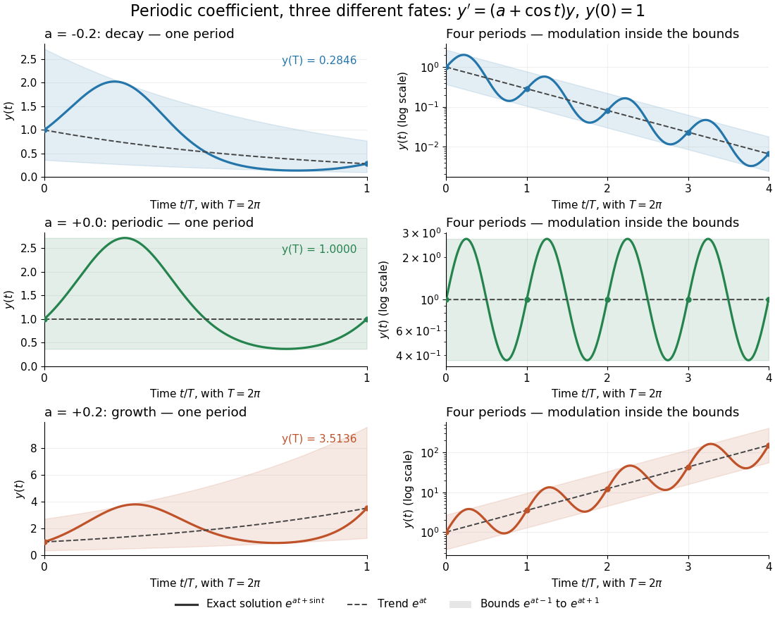
One repeating coefficient can produce decay, periodic motion, or growth
. The original example , , shown over one coefficient period and four coefficient periods. Shading marks the bounds , and dashed curves mark . The right column uses a logarithmic vertical scale. Details.The exponential function separates two roles:For , even the decaying case initially rises, because . The growing case has intervals of decline, because becomes negative. This is the distinction between the instantaneous logarithmic derivative and the Floquet growth rate measured over many periods.
More generally, for a real continuous periodic function of period , the scalar linear differential equation hasA nonzero solution of a differential equation is -periodic exactly when , or equivalently when the coefficient has zero integral over a period. This scalar calculation is the simplest example of a Floquet multiplier.[ref]
Differentiating a smooth characteristic flow map in its initial point gives this linear equation, with . The Liouville formula for a fundamental matrix then gives . Incompressible Hamiltonian flows preserve Lebesgue measure because this divergence vanishes.
If a continuous nondecreasing modulus satisfies this divergence condition, an estimate with locally integrable gives uniqueness of characteristic curves. Apply a regularized integral comparison to their separation. For the log-Lipschitz modulus, gives while . Zero initial separation stays zero. Unlike the usual linear Gronwall inequality, this criterion allows non-Lipschitz vector fields.
For a nonzero constant-coefficient polynomial differential operator in one variable, every homogeneous distribution solution is a classical solution, indeed analytic. Factor the polynomial into powers of distinct characteristic roots of a constant-coefficient differential equation. The kernel decomposition for coprime polynomials reduces the equation to , and multiplication of a distribution by a smooth function reduces this to . The fact that a distribution with zero derivative is constant, iterated, makes the latter distribution a polynomial of degree less than .
For a positive-order constant-coefficient ordinary differential equation, the kernel of multiplication by a coordinate gives exactly when . Hence every solution is , where and is any fundamental solution of a linear differential operator. Taking a retarded fundamental solution of a constant-coefficient ordinary differential operator shows that the extra freedom is a single jump in the derivative of order one below the operator order. The coordinate multiplies the already differentiated distribution: this is a different operator from .
If a degree- characteristic polynomial has distinct roots of a polynomial of multiplicities , all homogeneous distribution solutions are the displayed combinations. There are independent coefficients. Repeated characteristic roots of a constant-coefficient differential equation account for the polynomial factors multiplying exponentials; conjugate pairs give real sine and cosine combinations when real solutions are desired.
An implicit solution describes a solution of a differential equation through a relation , instead of isolating in an explicit formula. The relation describes a level set; an actual scalar solution of a differential equation must be a differentiable function on an interval whose function graph lies in the equation's domain. A whole level set need not be one such function graph.
For example, considerImplicit differentiation of gives . For , the circle contains two solutions of a differential equation,Both satisfy the equation on the stated open interval, and their function graphs stay in . An initial condition fixes and selects the sign of . In particular, gives and the upper branch on . The constant alone does not select the branch.[ref]
1.3 Separable equations. §1.3.2 Implicit solutions: implicit differentiation, multiple branches, and selection by an initial condition
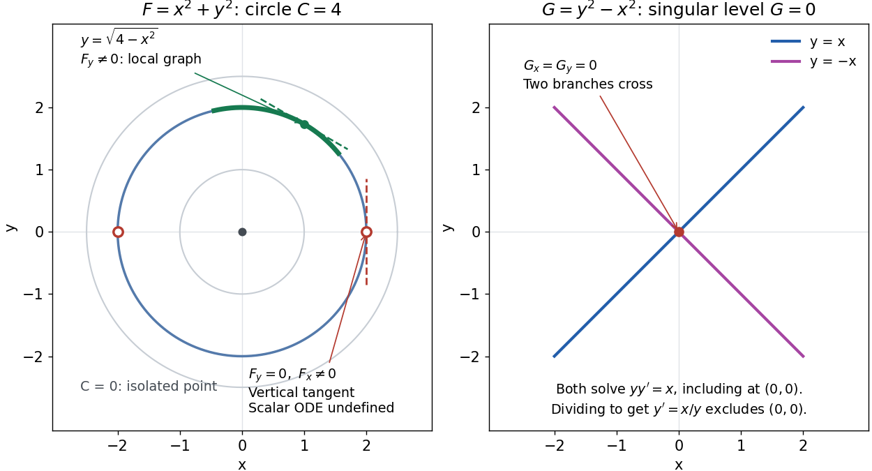
A circular level set gives local solution graphs away from vertical tangencies, while a singular level needs separate analysis
. Details. The precise local criterion uses the implicit function theorem. Let be continuously differentiable on an open subset of the plane, with . If its partial derivative , the nearby level set is a unique continuously differentiable function graph through that point. The chain rule givesThis proves that the local function graph solves there. For a different prescribed equation , one must also check along that branch and that it stays in the domain of . A level set by itself does not verify an arbitrary ordinary differential equation.[ref]
8.5 Inverse and implicit function theorems. §8.5.1, Theorem 8.5.6 and the preceding circle example: local existence, uniqueness and derivative of an implicit graph
For , the upper branch through has and tangent line slope . At , however, and . The circle remains a smooth regular level set with a vertical tangent line: it can be written locally as , but not as a single function graph over an open interval containing . Moreover, is undefined there, so the scalar solution of a differential equation cannot include this point in its domain. Changing the parameter draws the curve through the point but does not extend that scalar initial value problem.
When both partial derivatives vanish, even the geometry needs separate inspection. The level is an isolated point, not a function graph on any nonempty open interval. The zero level set of instead consists of the two lines and crossing at the origin, where . Each line satisfies the implicit ordinary differential equation , including at the origin; the explicit form excludes the origin. Thus algebraically dividing by a vanishing coefficient changes the domain and can change which solutions of a differential equation are admissible. Vanishing alone is only failure of a sufficient test: has the smooth zero function graph despite everywhere on it.
Implicit solutions are especially useful for exact first-order ordinary differential equations and for finding a first integral of an ordinary differential equation: a conserved relation can reveal allowed states without an explicit formula. For the normalized harmonic oscillator written as , , the energy has . Its positive level sets are the same circles. Where , eliminating time gives and the local implicit solution above. The harmonic oscillator's parametric curve continues through because its vector field governing evolution in time is defined there; treating as the independent variable fails at that turn. The origin is an equilibrium point of the harmonic oscillator, although it is excluded from the scalar equation .
An equation is exact if is an exact differential form: there is a potential with and . Its solution curves are levels . For continuously differentiable coefficients, suffices locally and globally on a simply connected domain. Global topology matters; a closed form on a punctured domain need not be exact.
On a common compact solution domain, a right-hand side continuous in parameters and uniformly Lipschitz in the state yields continuous dependence of the solution on those parameters. The Gronwall inequality controls the difference of two solutions. A transverse zero of an event function persists under a small parameter change, which allows a simple stellar surface in the Newtonian limit to persist in relativistic models.
For a stable first-order linear equation , the time is the interval over which a deviation from equilibrium decays by the factor . This is the dynamical exponential-decay sense, distinct from a Markov chain's spectral relaxation time.
An initial value problem combines an ordinary differential equation with an initial condition, for example and . The task is to find a solution of a differential equation on an interval containing which has that starting value. For a continuous linear differential equation , every prescribed finite vector determines a unique solution on the coefficient interval. A boundary value problem can instead prescribe values at distinct endpoints.
For the cooling initial value problem , , where and are constant, the unique solution isTake degrees Celsius, degrees Celsius, , and per minute. Then degrees Celsius. Reaching degrees Celsius requires , so minutes. The time constant minutes reduces the excess temperature by a factor ; it does not reduce the absolute temperature by that factor.
Uniqueness needs assumptions. If is a continuous function on an open neighborhood of and satisfies a local Lipschitz condition in , uniformly in , the Picard-Lindelöf theorem gives a unique local solution. Concretely, a finite bounds in a sufficiently small rectangle. Cooling satisfies this with . Local existence does not promise existence for all future time: , , has on and finite-time blowup at .
Continuity alone is insufficient for uniqueness. Consider the dimensionless initial value problem involving a square root and an absolute value:Besides , each delay gives a solution for :At , delays give , despite identical starting data. These are valid solutions of a differential equation: for , both one-sided derivatives at the join are zero; for , the right derivative at the starting time is zero. After the join, because . Squaring alone would also suggest a parabola before the join, but its negative derivative there would violate the equation. Since , a forward solution starting from zero stays nonnegative.
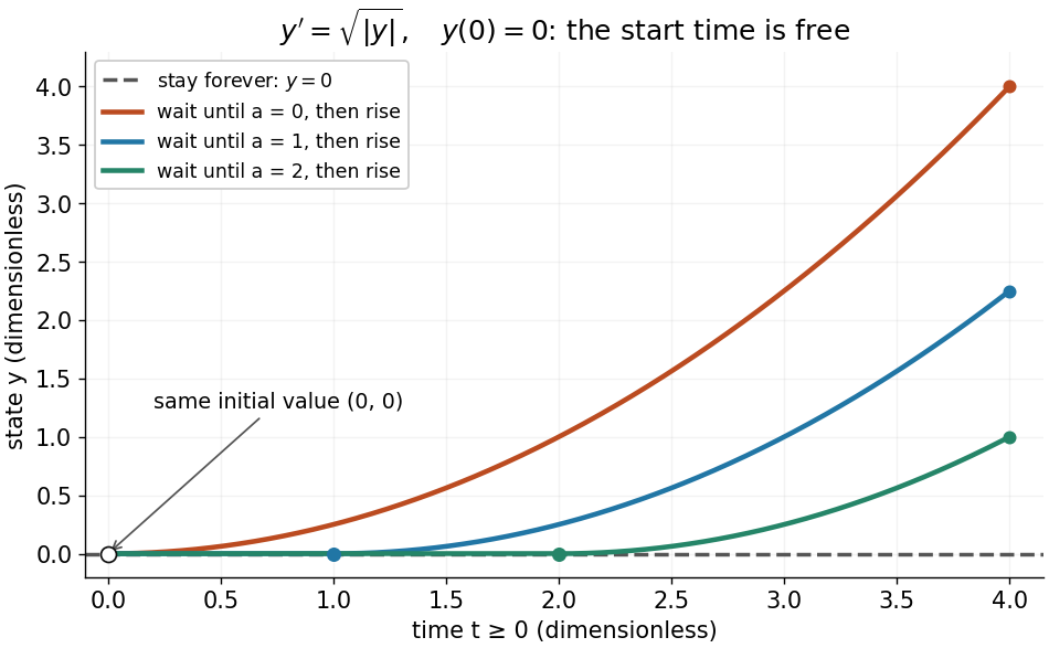
One initial value permits infinitely many delayed-start solutions without a Lipschitz condition
. Details. The right-hand side is a continuous function but fails the Lipschitz condition at zero: for , is unbounded. Thus the Peano existence theorem still supplies local existence, while the Picard-Lindelöf theorem does not supply uniqueness. Related waiting-time examples and a sufficient uniqueness condition appear in MIT 18.034, Lecture 2: Fundamental Principles.
A brief proof outline explains the mechanism: rewrite the initial value problem as the integral equation . On a short enough interval, the Lipschitz condition makes the right-hand side a contraction mapping on a closed set of continuous functions near . The contraction mapping theorem gives a unique fixed point; the fundamental theorem of calculus turns it back into a solution.
The displayed implicit ordinary differential equation has a singular initial point at the origin. On a nonconstant regular branch, treating as a function of gives . The integrating factor yields the first integral of an ordinary differential equationOne can verify this identity without dividing by : its derivative along a solution is .
The initial point forces , so . Near the origin this gives the two differentiable solutions and , with initial slopes zero and one. A division by would lose the first solution. A piecewise switch between the two at zero would fail differentiability because their one-sided slopes differ.
There is no conflict with the Picard-Lindelöf theorem: solving explicitly for requires division by , which vanishes at the initial point. A regular implicit equation or a local uniqueness theorem must be checked before claiming a unique solution through a singular point.
An L2 initial condition specifies a square-integrable initial function up to equality almost everywhere. It need not have pointwise nodal values or classical derivatives. L2-compatible initialization of grid data uses bounded averaging or projection, and evolution estimates use the relevant L2 norm.
A degenerate ordinary differential equation has a highest-derivative coefficient that vanishes somewhere in its domain. Its solutions can have lower regularity at that point than in the interior. A boundary value problem normally imposes endpoint values by continuous extension while requiring the differential equation in the interior. Requiring it pointwise at a degenerate endpoint with all derivatives finite can impose an extra condition and destroy existence. In a square-root-degenerate endpoint layer, the product of a vanishing square-root coefficient with a diverging second derivative has a finite nonzero interior limit.
An equation can remain meaningful at a zero of even though its normalized second-order linear differential equation has singular coefficients. A global continuation problem must specify its solution regularity. Across a point where a homogeneous solution vanishes to second order, its coefficient may change in a piecewise continuation; requiring continuity of the second derivative can eliminate that freedom. The usual continuous-coefficient uniqueness theorem for ordinary differential equations cannot simply be applied across such a point.
Use . For a nonzero one-variable polynomial and , a compactly supported solution to exists exactly when annihilates every smooth solution of the transposed equation . For simple roots , these test solutions span the exponentials , so the condition is . Dividing the entire transform by and applying polynomial division preservation of exponential type and the Paley–Wiener–Schwartz theorem constructs the compactly supported solution. It is unique because an entire function killed by a nonzero polynomial must vanish identically. For a root of multiplicity , the conditions become for , corresponding to .
A real vector field is dissipative in an inner product iffor all . Two solutions of the ordinary differential equation satisfyThus their distance never increases. The linear case recovers the dissipative operator condition. B-stability asks whether a Runge-Kutta method preserves this contraction for every positive step size.
Let be an open set, , and a continuous function. Through every there is a local solution of a differential equation: a continuously differentiable function on an open interval containing , satisfying the displayed initial value problem pointwise. No Lipschitz condition is assumed.[ref]
Ordinary Differential Equations and Dynamical Systems by Gerald Teschl. Gerald Teschl, Ordinary Differential Equations and Dynamical Systems, §2.7, Theorem 2.19, printed p. 56: forward existence and the analogous backward result
Continuity of a proposed rate law therefore guarantees at least one trajectory for a short time. For a physical model, this is a first consistency check: can the stated rule and initial condition actually be followed? Prediction also needs uniqueness. The delayed solutions of a square-root differential equation below show how the same rule and initial condition can leave a departure time undetermined. The Picard-Lindelöf theorem supplies a sufficient additional hypothesis for uniqueness; failure of that hypothesis alone does not prove nonuniqueness.
For the initial value problem , , a forward solution of a differential equation can stay zero until any , then follow . The delayed solutions of a square-root differential equation verify this freedom exactly.
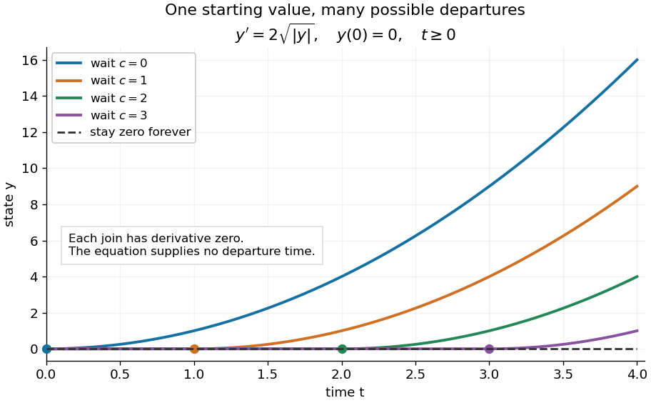
One initial condition admits an arbitrary forward waiting time
. Colored curves leave zero at the marked waits ; the dashed curve stays zero forever. Every curve satisfies the same original differential equation for . Details.Local existence gives neither a global solution of a differential equation nor a bound on all future values. The continuous function already permits finite-time blowup; the finite-dimensional continuation criterion explains the additional issue of extending a trajectory within its domain.
Proof outline: choose a compact set . By the extreme value theorem, . Take with . Forward Euler method polygons remain in the closed ball and satisfy . The Arzelà-Ascoli theorem yields a convergent subsequence with uniform convergence. Uniform continuity of on makes their integral equation defect tend uniformly to zero, so the limit satisfiesThe fundamental theorem of calculus gives a continuously differentiable function. Repeat backward and join at , where both derivatives equal .[ref]
The compact set here uses a finite-dimensional vector space; bounded closed balls in an arbitrary Banach space need not be compact. When , the constant solution of a differential equation works on the entire time interval in . In general the proof selects a subsequence, without asserting that all polygons converge to one unique trajectory.
This initial value problem uses a square root and absolute value to define a continuous function on all of . For every finite waiting time , a forward solution of a differential equation on isThe constant solution of a differential equation is another choice. For example, at , waits give values . These are dimensionless mathematical trajectories; no measured physical waiting time is being supplied.
Verification uses the original ordinary differential equation, including the join. Before departure, both and vanish. For , their common value is . For , the difference quotient at the join isThus the derivative exists at , equals the rate law there, and is continuous across the join. For the same computation gives the right derivative at the starting endpoint. For , the left and right second derivatives at departure are and : these forward solutions of a differential equation are continuously differentiable functions, without being twice differentiable at departure. The local two-sided statement of the Peano existence theorem is separate from this explicitly forward family.
The rate law tends to zero as , but its secant slopes from zero are unbounded:No finite local Lipschitz constant exists at zero. At the quotient is , even though the rates are shrinking to zero. Continuity controls the rate itself; Lipschitz continuity would control its change relative to the state displacement.
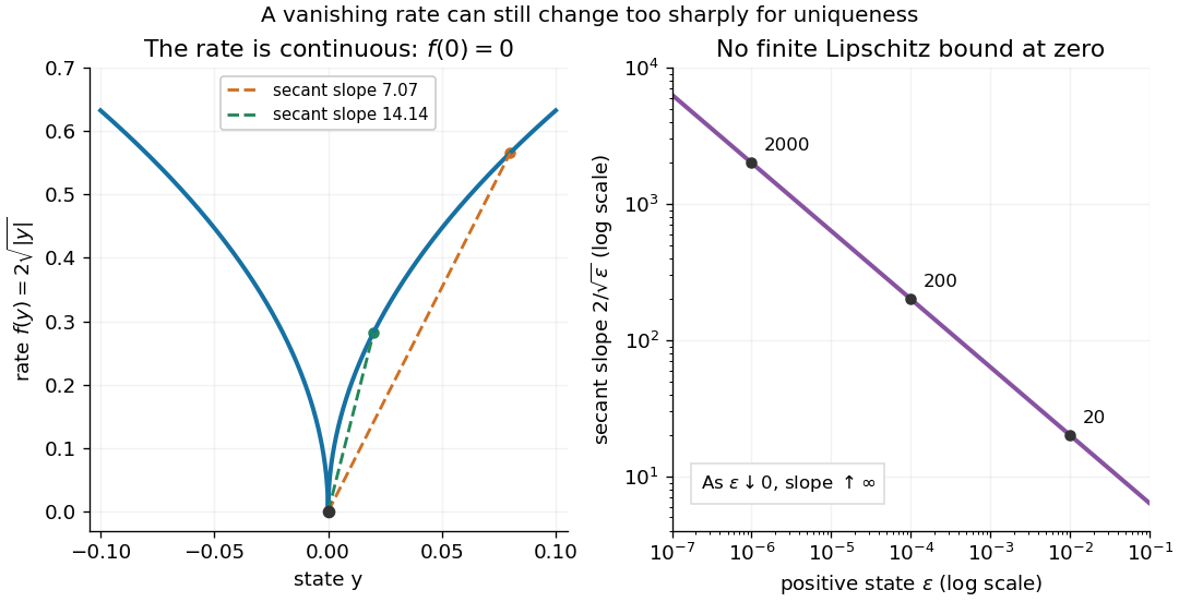
There is also a numerical lesson. The forward Euler method starting exactly at zero gives at every step. It reproduces the constant solution of a differential equation for every positive step size, while the moving trajectories remain equally valid. A computation producing one trajectory cannot establish uniqueness. Likewise, the separable differential equation calculation that divides by only describes the moving pieces: checking the original equation recovers the zero pieces and their joins.
For the autonomous differential equation , the real solutions are nondecreasing and lie in . On each nonconstant interval, separation of variables gives , so the solution crosses from to in exactly time . Every nonconstant solution on the entire real time axis is consequentlyfor some real . The two constant solutions complete the list; solutions on shorter intervals are restrictions of these. At the joins both the derivative and the right-hand side are zero, so these are continuously differentiable functions. The right-hand side is continuous but fails Lipschitz continuity at both endpoints, allowing arbitrary waiting time at before departure. Once reaches , monotonicity forces it to stay there. The sine representation without the nonnegative-cosine restriction would incorrectly introduce decreasing pieces.
A first-order ordinary differential equation is separable if its explicit form factors as . On an interval where , write and take antiderivatives to obtain an implicit solution:An initial condition determines and selects a branch and domain. The useful simplification is that the two integrals each involve only one variable, even when the original equation is nonlinear.
For Newton's law of cooling, division by gives . To keep the logarithm dimensionless, integrate relative to the initial excess temperature:When , continuity preserves the sign of the excess temperature until any potential zero, giving . This formula never reaches zero at finite time. Taking its derivative verifies the ordinary differential equation, and substitution at verifies the initial condition.
Always check what division removed. Each zero gives a constant solution of a differential equation . Cooling therefore also has the equilibrium point , omitted by division but included in the final explicit formula. For the nonunique initial value problem , division by only describes the moving pieces: a valid solution may remain zero for an arbitrary time before joining one. Separation is a method for finding solutions, not a uniqueness theorem.
The product rule gives for , reducing the displayed equation to the autonomous separable differential equation . On an interval where , integrate and recover for . Zeros of give additional constant solutions for and must be considered before division. A solution for extends through zero only if the recovered quotient has the necessary finite derivatives and satisfies the undivided original equation there.
The substitution turns the nonzero solutions into . Thus where the denominator is positive, together with . The nonzero equilibrium points are attracting and is unstable. The sign of nonzero initial data is preserved.
A nonlinear ordinary differential equation depends nonlinearly on the unknown function or its derivatives: it cannot be written in the form defining a linear differential equation. For example, contains a square of the unknown function, and is a logistic differential equation. A coefficient such as depending only on the independent variable does not make an ordinary differential equation nonlinear. This distinction concerns dependence on the unknown, rather than the shape of its function graph.
For a concrete initial value problem, consider , . Its solution of a differential equation isTaking its derivative gives , and evaluating at zero checks the initial condition. The stated interval contains zero and ends at finite-time blowup: tends to positive infinity as approaches from below. Increasing the positive initial condition brings finite-time blowup closer. This is a simple mathematical example with dimensionless and , rather than a calibrated physical model.
Choose and , giving and . At they have values and , so their sum has value . On the common interval , both are valid solutions of a differential equation, but their sum fails the same ordinary differential equation:Already at , and its derivative is , whereas would require . At , the defect is . The cross term explains the failure of the superposition principle, even though each individual solution of a differential equation is a smooth function.
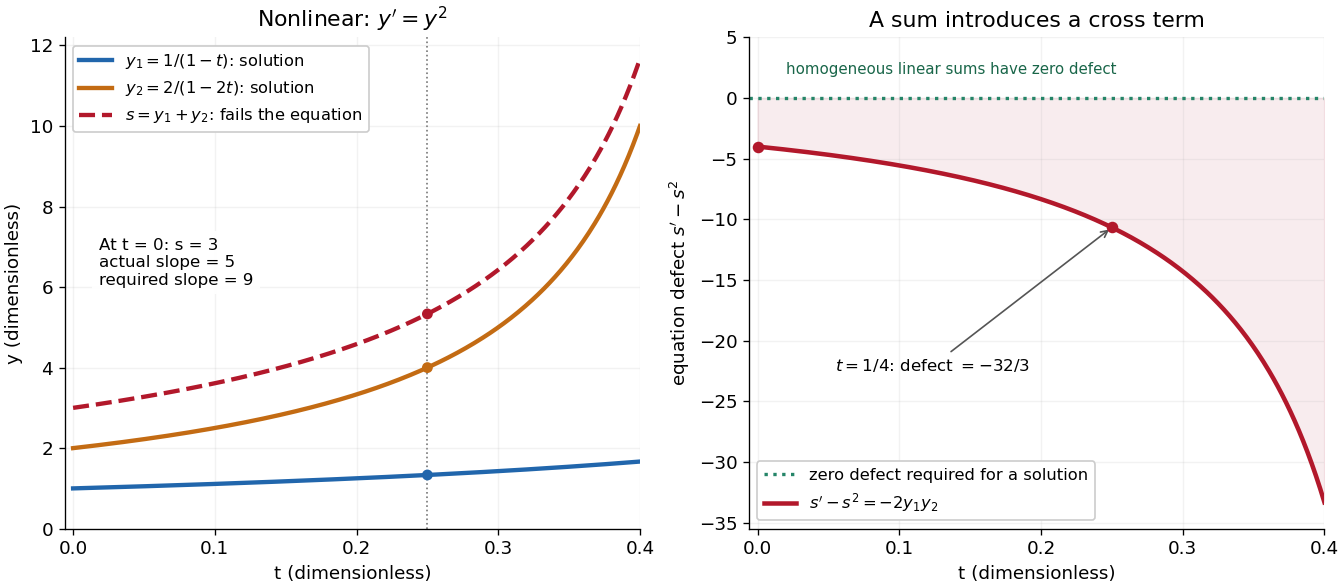
The first panel shows , and their invalid sum only up to , before either finite-time blowup. The second measures the defect in the ordinary differential equation, including the computed value at . For a homogeneous linear differential equation, the corresponding defect of a sum is zero. Nonlinear ordinary differential equations can describe state-dependent growth such as the logistic differential equation, whose negative quadratic term limits growth instead of accelerating it without bound. Recognizing the distinction tells us when we may assemble solutions of a differential equation from simpler pieces and when we must account for their interaction. See MIT's worked counterexample to nonlinear superposition.
This nonlinear ordinary differential equation governs the amplitude of a complex oscillator solution. Independent real solutions of can be combined into a nonvanishing complex solution; its modulus satisfies the equation with equal to the squared Wronskian. A real positive amplitude and a conserved phase flux give an exact representation, not merely a WKB approximation.
Substitution of into gives the displayed real amplitude equation and conserved imaginary-part flux. Conversely these equations produce an exact complex solution wherever . The WKB approximation is obtained by expanding this exact system where stays positive.
In , the damping coefficient depends on the displacement. The oscillator energy satisfies . Positive dissipates energy and negative supplies it; a changing sign can select a stable amplitude. The averaged amplitude for position-dependent damping measures the net effect over an oscillation.
The logistic differential equation is the nonlinear ordinary differential equationAs a mathematical model of population dynamics, it treats abundance as a continuous nonnegative quantity. The constant has units of inverse time, while the carrying capacity has the same units as . The useful idea is to combine growth resembling exponential growth at low abundance with a slowing approach to a finite abundance. The three trajectories below already show an important distinction: starting above the carrying capacity gives a decreasing curve, whereas starting below it gives an increasing one.
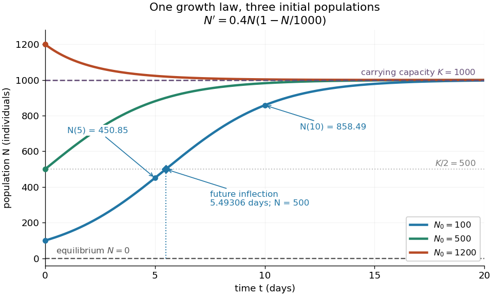
Logistic trajectories approach the carrying capacity from below or above
. Here and per day. The initial conditions are ; dashed horizontal lines show the two equilibrium points and . Only the trajectory has a future inflection point, marked at and days. The other marked values are and for that same trajectory. Details.For , dividing the derivative by abundance gives the instantaneous per-capita rate:It decreases linearly with : it approaches at low abundance, is at , vanishes at the carrying capacity, and is negative above it. This per-capita rate differs from the total rate , which also counts how many individuals contribute. It is an instantaneous rate, rather than a fixed percentage increase over a whole day. The linear per-capita assumption and the resulting qualitative picture are developed in MIT 18.03SC's logistic-model notes.
Writing , the equilibrium points satisfy , so the constant solutions of a differential equation are and . The phase line points upward for and downward for . Also and : the criterion for fixed point stability for an autonomous differential equation makes zero an unstable equilibrium and an asymptotically stable equilibrium point. Every positive initial condition approaches as ; stays exactly zero. Instability of zero means that a small positive population grows away from it, not that a zero population spontaneously appears.
For every , the unique solution of a differential equation for all isThe denominator is positive on this domain, including when . For , this is a translated and scaled logistic function; its extension to all real times is a sigmoid function. For the coefficient of the exponential function is negative, and the future curve instead decreases toward . No nonconstant positive solution of a differential equation crosses or reaches it at finite time. A short derivation uses the dimensionless variable : the chain rule gives , so exponential decay yields . The substitution divides by , so the zero equilibrium point must be included separately.
The total growth rate is a downward-opening quadratic function of abundance. Completing the square gives its maximum without solving the differential equation:The balance is beautiful: more individuals contribute to growth, but each contributes less, and the strongest total increase occurs halfway to the carrying capacity. This is a maximum over possible abundances. A trajectory starting above never passes through that abundance in its future.
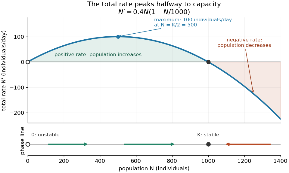
Total logistic growth is greatest at half the carrying capacity
. With and per day, the maximum is individuals per day at . The function graph crosses zero at the equilibrium points and ; beyond the rate is negative. The lower phase line has arrows toward increasing abundance below and toward decreasing abundance above , with a hollow mark for the unstable equilibrium and a filled mark for the asymptotically stable equilibrium point. Details.The chain rule connects this maximum to the shape of the time trajectory through its second derivative:For , the trajectory initially has convexity and then concavity, with its one future inflection point atFor , this point lies at the initial time, with concavity for . For , the inflection point belongs to the past extension, so the future trajectory has concavity throughout. Above , the decreasing trajectory has convexity and no inflection point. The two constant solutions of a differential equation have no change of concavity. Thus an entire logistic function has an S shape, but its observed future segment need not show both bends. See also [ref].
For the plotted example with , and , time measured in days givesThe initial total rate is individuals per day, and the initial per-capita rate is . The fastest total increase is individuals per day, reached at days. At that time the per-capita rate has already fallen to .
These parameters are illustrative choices, rather than an empirical fit. The equation specifies deterministic evolution under a phenomenological assumption: it summarizes how net growth depends on abundance without separately modelling every process that affects it. The carrying capacity is a parameter for a specified setting, not a universal constant for all populations. In his 1838 paper "Notice sur la loi que la population suit dans son accroissement", Correspondance mathématique et physique 10, pp. 113–121, Pierre-François Verhulst proposed , equivalent to this equation with and . He also noted that different assumed growth-retarding terms could describe the observations similarly while giving very different limiting populations. This is an early illustration of why a good-looking curve alone does not establish a unique long-term prediction.[ref]
https://www.neo-classical-physics.info/uploads/3/4/3/6/34363841/verhulst_-_law_of_population.pdf. Verhulst's 1838 paper, translated by D. H. Delphenich
The logistic differential equation describes continuous time. The logistic map instead advances in discrete steps and can exhibit a period-doubling cascade and Devaney chaos; the monotone positive trajectories here cannot. Their connection through the forward Euler method is explained under Euler discretization of logistic growth, where a large step can introduce behaviour absent from the original differential equation.
The forward Euler method applied to the logistic differential equation becomes the logistic map after , . The positive equilibrium point of the differential equation has perturbations decaying as . Its discrete fixed-point multiplier is : for , the discretization has an artificial oscillatory instability, leading initially to alternation on successive steps. This contrasts with the positive perturbation multiplier of the exact time-step map.
Let be an open set and a continuous function. Suppose is locally Lipschitz in the state , with a Lipschitz constant uniform on a sufficiently small time-state neighborhood of each point. Then each determines a unique local solution of a differential equation to the displayed initial value problem, on an interval around . This is the local theorem in Ordinary Differential Equations and Dynamical Systems by Gerald Teschl.
For example, , , has the solution of a differential equation : its derivative is itself and its starting value is . The Lipschitz constant is , since . Thus uniqueness follows even before computing . Picard iteration below constructs this exponential function one polynomial at a time.
The Lipschitz condition has real content. For the continuous function involving a square root,each waiting time gives a different forward solution of a differential equation:The constant solution of a differential equation is another choice. At , delays give respectively. Before the join, both sides of the ordinary differential equation are zero; afterwards, . Both one-sided derivatives at are zero, so the join is valid. All these trajectories can also be extended by zero to . The failed Lipschitz condition is visible in the quotientFor this quotient is . Continuity still allows local existence by the Peano existence theorem; it cannot choose a waiting time. MIT's 18.034 Lecture 2, Example 2.3 develops the same waiting-time mechanism for a different ordinary differential equation, .
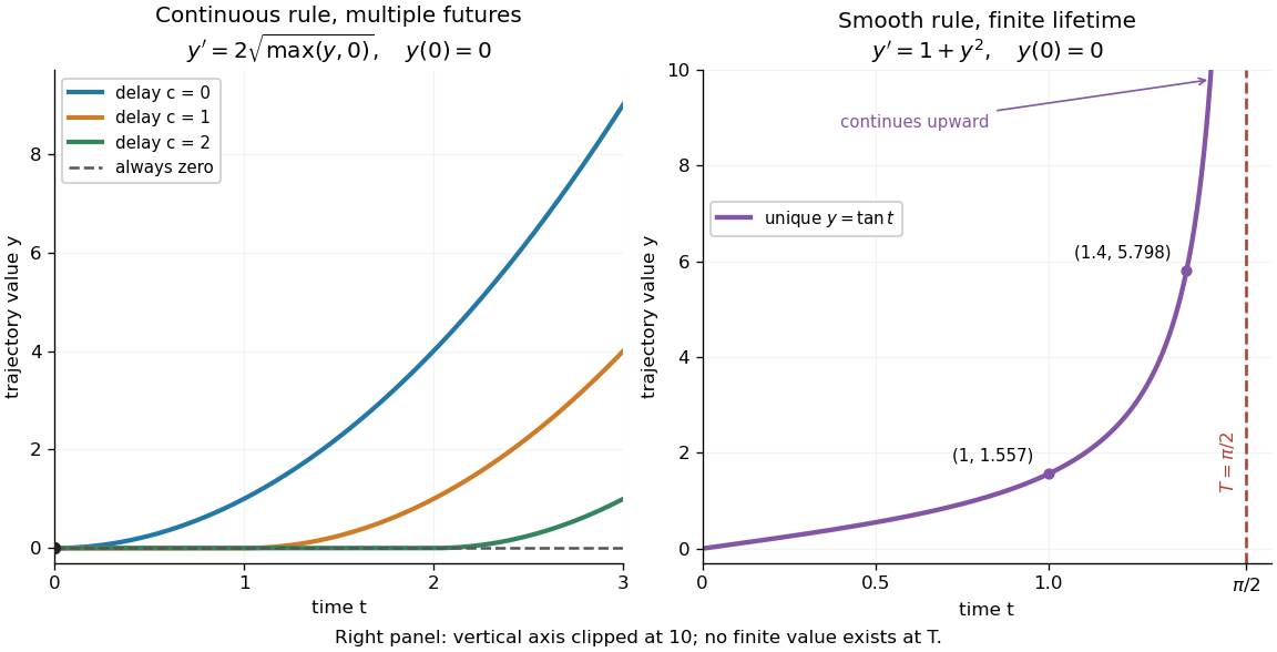
Failure of uniqueness and finite-time blowup are different obstructions
. Left: several delayed solutions of a differential equation of share . Right: the unique solution of a differential equation of , , has finite-time blowup at . The right vertical axis ends at ; the curve continues upward beyond the plot, and there is no finite endpoint value. Details.The useful promise is that an initial condition and a sufficiently regular local rule select one trajectory. It justifies comparing models and following trajectories without an arbitrary choice at each instant. A locally Lipschitz continuous rule need not keep that trajectory bounded: meets the theorem's hypotheses everywhere but has finite-time blowup. Longer existence is governed by the finite-dimensional continuation criterion.
For the ordinary differential equation through , consider a symmetric existence rectangle , . Its maximum slope bound is . The condition becomes . Differentiating shows its maximum occurs at , givingThis is the largest interval guaranteed by this particular centered-rectangle criterion. Direct separation of variables instead gives on the maximal real interval . The comparison shows the difference between a sufficient local existence theorem and the actual continuation interval. The endpoint obstruction is the zero of the denominator at .
A coefficient that vanishes at the initial time can hide failure of the uniform Lipschitz condition required for an initial value problem. For , the map is identically zero. But every rectangle of positive widths around contains some , andNo Lipschitz constant works uniformly on the rectangle. Actual uniqueness also fails: and are distinct differentiable solutions with initial value zero. Substitution gives for the second solution. A condition at the single initial time cannot replace control on a neighbourhood.
Suppose is continuous and Lipschitz in its state variable on a closed cylinder , , with bounds and Lipschitz constant . On a smaller interval of radius , the displayed Picard operator maps continuous curves in that closed ball into itself when , and it is a contraction mapping in the supremum norm when . This function space is complete because it is a closed subset of a Banach space of continuous vector-valued functions. The contraction mapping theorem gives a unique fixed point, and the fundamental theorem of calculus makes it a solution of the ordinary differential equation. Choosing also prevents any solution with the same initial data from first exiting the cylinder during that interval.
For the autonomous differential equation , the displayed family stays at until time and then decreases below it. Here . Direct differentiation verifies the equation on each side; since , the derivative tends to zero at departure, making the joined function continuously differentiable. Distinct departure times give different solutions from the same equilibrium initial condition. The ratio is unbounded, so the local Lipschitz continuity hypothesis of the Picard-Lindelöf theorem fails.
A solution starting above reaches it in finite time. It can then use any of these continuations. For , , and initial value , arrival occurs at time two; departure at gives afterwards. Waiting-time solutions of a sublinear Bernoulli equation give a related mechanism for departures in the opposite direction.
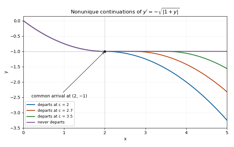
Different waiting-time continuations at a non-Lipschitz equilibrium share the same earlier trajectory
. Details. Picard iteration replaces a tentative trajectory by the accumulated integral of its proposed rate. For an initial value problem , , define the Picard map and its starting function byHere is the constant starting trajectory; the same symbol without its argument denotes the initial state. A fixed point of solves this integral equation, and the fundamental theorem of calculus gives the original ordinary differential equation.
For , , successive integrals giveAt , the first five values are , while . The fourth polynomial misses by about . On , every omitted term of the exponential series is nonnegative and increasing, so the largest error occurs at . The tail tends to zero, giving uniform convergence to the exponential function on this interval.
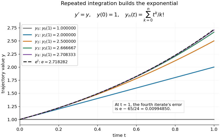
Picard iteration builds the exponential solution by repeated integration
. The first five polynomials approach the exponential function on . Endpoint values are listed in the legend; the last error is approximately . Details.The beauty of Picard iteration is that each proposed trajectory supplies a better rate history for the next one. For this example, one integration adds exactly the next term of the exponential series. In general, the integrals may be difficult to compute, but the construction still explains local existence and uniqueness.
The short contraction mapping argument needs two independent controls. Choose a time-state cylinder on whichThe second bound is the uniform local Lipschitz condition. Set with , and . In the function space of continuous functions , use the supremum norm . On its closed ball , direct integral estimates giveThus the map preserves the closed ball and is a contraction mapping there. This closed ball is a complete metric space, so the contraction mapping theorem gives convergence to exactly one fixed point. Any other local solution of a differential equation stays in the same ball after shortening its interval, and hence agrees there.
For , take , so in the state ball and , . Choosing gives and , with the actual solution satisfying . The plotted interval is longer than this simple guarantee: the explicitly computed exponential series converges there anyway. The condition is sufficient for this one-step contraction mapping argument, rather than a necessary lifespan bound.
For real constants , apply Picard iteration to the initial value problem , , starting with . The recurrence isSince , mathematical induction gives the displayed partial sums. The exponential series converges at every finite argument, so for every real , uniformly on each compact interval in that range. This is not a Taylor series in , so its convergence is not restricted to . The differential equation's coefficient is singular at even when a special solution has a removable singularity there.
For Picard iteration , , assume and a Lipschitz constant on a rectangle containing every iterate. The first difference is at most . Integrating the preceding bound multiplied by proves the displayed estimate by mathematical induction. Its uniform bounds sum to a convergent exponential series for every finite , so the Weierstrass M-test gives uniform convergence without requiring .
For two arbitrary initial functions in a function set preserved by the Picard iteration operator , the same induction givesThus some iterate is a contraction mapping on any fixed finite interval for which every iterate stays in that set. The iterated contraction argument gives a unique fixed point of on a nonempty complete metric space, without requiring . For a rectangle with field bound and vertical radius , supplies the required self-mapping property.
Consider the Volterra integral equationwhere is continuous, , , and the continuous kernel satisfies for , with . If , there is exactly one continuous solution on the whole half-line. It is bounded, and Picard iteration beginning at converges in supremum norm with contraction ratio at most .
For a proof, the integral of the kernel is at most . Thus maps the closed ball of radius in the Banach space of bounded continuous functions into itself, since . Factoring gives on this ball. The contraction mapping theorem gives its unique fixed point. A first-exit argument shows that every continuous solution, even one not initially assumed bounded, stays strictly inside the same ball: a first time with would contradict . Reapplying the estimate gives the strict global bound , so uniqueness is unrestricted within the continuous solution class. If , zero is the only solution by the Gronwall inequality on each finite interval.
A Picard iterate is one of the successive approximate solutions of a differential equation obtained by repeatedly applying its integral solution operator. If and , the usual operator is . An integrating factor can produce a different, equivalent operator with better estimates, as in Global Picard iteration with a decaying kernel. The word iterate denotes an approximate function; Picard iteration denotes the procedure.
Under the Picard-Lindelöf theorem's hypotheses on , extend a solution of a differential equation as far as possible, to a maximal interval . If , the time-state trajectory must eventually leave every compact subset of . Equivalently, confinement near to one compact subset of permits continuation past . See Teschl, Section 2.6, Lemma 2.14 and Corollaries 2.15–2.16, pp. 52–53.
The domain restriction matters even for a bounded trajectory. Restrict , , to . Then exists in this domain only for ; at its values are . As , it approaches the excluded boundary point while remaining bounded. Its trajectory cannot fit into any compact subset of near that endpoint. This is escape from a finite domain, without finite-time blowup in norm. Enlarging the domain to gives the same formula for every real .
Conversely, , , stays in the compact set for every fixed . Its growing exponential function is unbounded over the entire future, but has no finite-time blowup. At , its largest value on is only . The relevant question is boundedness before each finite endpoint, rather than one bound valid forever. The tangent function in the diagram under the Picard-Lindelöf theorem illustrates the other possibility: its norm escapes every bound before .
This criterion is useful because an estimate can secure continuation without an explicit formula. In a finite-dimensional vector space, a bounded closed ball is compact; a bounded state trajectory therefore supplies the needed compact set when its time-state closure is inside the domain. That final proviso prevents mistaking a domain boundary for finite-time blowup.
A common sufficient estimate comes from global Lipschitz continuity in the state. Assume for an open time interval , with continuous and a Lipschitz constant valid for all states on each compact time interval under consideration. For , let , finite by continuity. Then , and the Gronwall inequality gives, for wherever the solution already exists,For instance, , , has and the exact solution , attaining this estimate; at the value is . Finite bounds of this kind give continuation throughout , with the analogous estimate backwards in time. When , this gives existence for all real times. If has a finite endpoint, it gives no continuation beyond that prescribed domain. The underlying linear-growth criterion is [ref].
A brief explanation of the continuation mechanism suffices: within the protecting compact set, the continuous function is bounded, say by . The integral equation yields near the finite endpoint, so has a limit . The protecting compact set puts inside . Restarting the initial value problem there and using local uniqueness joins the trajectories.
On , an exponentially or polynomially weighted sup norm can make a Volterra integral operator contractive even when the ordinary sup norm does not. For integration from to , the weight gives contraction factor at most for an -Lipschitz vector field.
A solution of a differential equation has finite-time blowup in norm when as approaches a finite endpoint of its maximal interval of existence. This is stronger than merely approaching an excluded boundary of an open state domain while staying bounded. The finite-dimensional continuation criterion distinguishes these obstructions; for a locally Lipschitz continuous ordinary differential equation on , a finite maximal endpoint inside necessarily entails finite-time blowup.
A simple example with a smooth right-hand side isThe derivative identity verifies the equation and the initial condition. Also for , giving local Lipschitz continuity and therefore uniqueness. Yet the positive blowup time is . Computed values show the accelerating growth:The right panel under the Picard-Lindelöf theorem deliberately clips its vertical axis at : the trajectory has already left the picture at , before reaching . A plot ceiling is a display limit, not a finite value at blowup.
The tangent function also quantifies the last part of the trajectory. With ,Thus the height is approximately the reciprocal of the remaining time. At remaining times , the heights are approximately . These follow from the sine and cosine limits at zero and explain the steep rise without relying on the appearance of a clipped function graph.
The distinction is useful when interpreting a solution of a differential equation: uniqueness certifies a trajectory while it exists, while growth estimates decide how far it can be followed. For , the Lipschitz constant on a bounded state interval grows with , and the right-hand side grows quadratically. There is no global Lipschitz constant or linear-growth bound of the kind used by the finite-dimensional continuation criterion. Smoothness at every finite state is entirely compatible with finite-time blowup.
A scalar linear differential equation of order has the formHere the coefficients and the forcing term are prescribed functions of the independent variable . A classical solution of a differential equation is an -times differentiable function satisfying the identity at every point of its interval. The unknown function and its derivatives enter to the first power, without products between them or coefficients depending on . Equivalently, the differential operator is a linear map: for constant scalars ,The forcing term may be zero, giving a homogeneous linear differential equation, or nonzero, giving an inhomogeneous linear differential equation. Linearity of does not mean that every function graph of a solution of a differential equation is a straight line.
To use the usual order- initial value problem theory on an interval , assume that throughout and that all and are continuous functions there. Dividing by normalizes the highest derivative; specifying at then selects one solution of a differential equation throughout . A zero of needs separate analysis: one cannot divide through it and retain these conclusions. The first-order normalization appears in OpenStax's definition and standard form of linear equations; the corresponding system theorem is in MIT's existence and uniqueness notes for linear systems.
The coefficients need not be linear functions of . For example, is a linear differential equation on , although is quadratic. Its solution of a differential equation with initial condition is : its derivative is , so substitution gives , and . The zero of the highest coefficient at explains the domain restriction. In contrast, , and are nonlinear ordinary differential equations because of their dependence on the unknown function. Variable coefficients and nonlinear ordinary differential equations are different issues; see MIT's definitions and examples of first-order linear equations.
The practical benefit of linearity is that it separates the effect of the initial condition from the effect of the forcing term. Once one particular solution satisfies , every solution of a differential equation isHere is the kernel of a linear map, consisting of solutions of a differential equation to the associated homogeneous linear differential equation. Indeed, , and conversely . Thus the family for a fixed forcing term is an affine space obtained by translating . If is not identically zero, the zero function is absent, so this family is not a vector space under the usual operations on functions. This short argument explains why a general solution is a particular solution plus a homogeneous solution.
A vanishing highest-derivative coefficient can make the two initial values of a second-order differential equation dependent. Suppose is continuous at zero, is constant, and a solution of has finite continuous at zero. Integration givesRegularity forces . Dividing by and taking the limit gives , since the integral average tends to . The remaining equation is first order and therefore has only one free regular initial value. For and , it yields and . This explains the reduced constant count without treating the singular endpoint as an ordinary second-order initial point.
In a fixed frame, a first-order linear differential equation is Fuchsian at a finite point when its coefficient matrix has at most a simple pole there. Its residue is . The global object is the matrix-valued one-form : in the coordinate its coefficient is . A Fuchsian system has intrinsic regular singular points, but an intrinsically regular singular system may have higher-order coefficient poles in a different meromorphic frame.
Suppose the matrix is holomorphic at zero and is an eigenvalue of . Let be the largest nonnegative integer for which is an eigenvalue of . Seek , with nonzero. The Frobenius method gives for , where scalar terms multiply the identity. Every left-hand matrix is invertible by the choice of . Its inverse is , so a scalar convergent majorant proves convergence of the series. This yields a nonzero analytic solution; it is necessarily nonconstant when , but can be constant when . For the displayed sign convention, indicial exponents are eigenvalues of .
A fundamental matrix for on a chosen logarithm branch is . A counterclockwise circuit changes the logarithm by , giving the displayed monodromy matrix and the cyclic group it generates. Changing the solution basis conjugates the matrix. The residue eigenvalues exponentiate to the monodromy eigenvalues; the latter do not determine the former uniquely.
For a system of linear differential equations , a fundamental matrix has columns forming a basis of its solution space. It solves and is invertible at every time in its interval. Every solution is for a constant vector : differentiating gives zero. Invertibility at one time implies invertibility throughout the interval by uniqueness of the initial value problem. This notion is distinct from a Markov-chain fundamental matrix or the projective-geometric matrix used in stereo vision.
Writing with an invertible matrix-valued function gives exactly when . For a formal power series transformation at an irregular singular point, coefficient comparison recursively removes off-diagonal terms when leading diagonal eigenvalues are distinct. This is a differential-system change of frame, not specifically an electromagnetic gauge transformation.
For , , the formal diagonal exponent has and . Matching the gauge equation gives the off-diagonal first coefficient and the diagonal one , where . The second coefficient has diagonal entries and off-diagonal entries . With and negative-index coefficients zero, the coefficient comparison isIts diagonal equations at give and the second diagonal coefficient respectively. Its off-diagonal equations determine the next coefficients because the commutator with multiplies the upper and lower entries by and . This proves the expansion and supplies the recursion for all higher orders. The generally nonzero supplies formal monodromy.
If and , differentiation of the determinant gives . For a planar periodic orbit this gives the nontrivial Floquet multiplier, since the tangent multiplier is one.
For a continuous periodic coefficient matrix , a fundamental matrix for , normalized by , obeys . The invertible matrix has a complex matrix logarithm; set and . Since commutes with , direct substitution gives and proves the factorization. A real logarithm is not required for this complex representation.
The eigenvalues of are Floquet multipliers. All solutions are bounded for forward time when every multiplier has modulus at most one and those on the unit circle have no nontrivial Jordan blocks. In a real undamped second-order scalar equation with no first-derivative term, the monodromy determinant is one. Distinct conjugate unit-modulus multipliers give bounded solutions; a nontrivial Jordan block at multiplier or gives an unbounded second solution even when one periodic or antiperiodic solution exists.
For a Floquet multiplier of a period- linear variational equation, a Floquet exponent is any logarithmic rate satisfying the displayed relation. Its real part is uniquely , while its imaginary part is defined modulo . Negative transverse real parts give local attraction to a periodic orbit; the autonomous phase direction has multiplier one and exponent zero. Constant-coefficient amplitude equations supply exponents directly as the eigenvalues of their Jacobian matrix.
The Floquet growth rate measures the exponential trend of a periodic linear differential equation over many coefficient periods. A Floquet multiplier measures the factor per period ; the corresponding rate per unit time iswhere is a Floquet exponent. Taking the real part removes the ambiguity in the complex logarithm.
For the scalar example under periodic solution, and the Floquet growth rate is , independently of . Indeed,The instantaneous logarithmic derivative keeps oscillating even though its average over complete periods is exactly . Sampling at the same phase in each period removes the modulation altogether: .
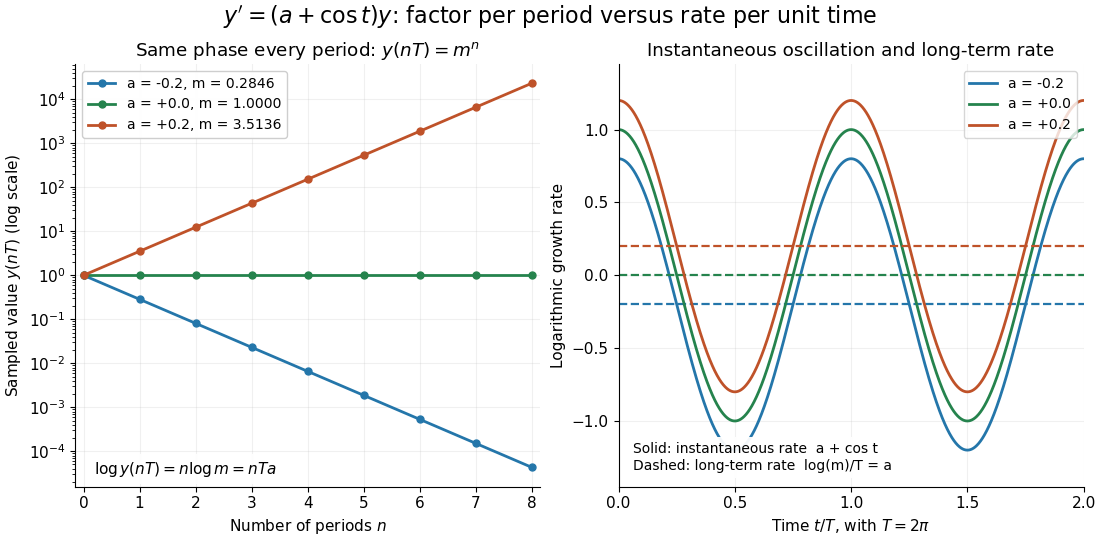
For the general finite-dimensional homogeneous linear differential equation , assume that is continuous on the real line and -periodic, with . Normalize its fundamental matrix by and set . The maximal asymptotic exponential rate, using any induced matrix norm, isHere is the spectral radius, are the Floquet multipliers, and invertibility gives . This concerns growth of the solution operator; it does not say that every initial condition attains the maximum.[ref]
To prove the formula, write with . Periodicity and uniqueness giveBoth and have uniformly bounded matrix norms on a period. Consequently differs from by at most fixed multiplicative factors. The spectral radius formula gives , proving the claimed limit without choosing a matrix logarithm.
For a particular nonzero initial condition , decompose into the generalized eigenspaces of over the complex numbers. The rate of is the largest among components that are nonzero. Generic data have a component in the dominant generalized eigenspaces and attain ; data contained in the sum of the subdominant generalized eigenspaces have a smaller rate. For example, with , the maximal rate is , while decays at rate . These invariant subspaces describe initial data at phase zero. Their transported versions can vary with time and satisfy .
A negative Floquet growth rate allows temporary amplification. For the constant non-normal matrixthe initial condition has Euclidean norm , which rises from to about at before eventually decaying. Its exponential rate is still : the Jordan block contributes a polynomial factor, whose logarithm divided by tends to zero. At a unit-modulus Floquet multiplier, such polynomial growth can even be unbounded with zero exponential rate; gives . Thus zero Floquet growth rate alone proves neither boundedness nor a periodic solution.
For the homogeneous linear differential equation with continuous coefficient matrix of period , the monodromy matrix of a periodic linear system is the one-period map from to . If is any fundamental matrix,Its eigenvalues are the Floquet multipliers. Multipliers are nonzero, since a fundamental matrix is invertible. Changing the starting phase conjugates , so the Floquet multipliers and Jordan blocks are independent of that choice.[ref]
This turns a continuous-time problem into repeated matrix multiplication:If , the associated solution of a differential equation obeys at every time, not merely at the sampled times. In particular, gives a nonzero -periodic solution, and every nonzero -periodic solution arises this way. If , the state changes sign after one period and repeats after two. A unit-modulus Floquet multiplier different from need not give repetition after one period, and a generalized eigenvector in a nontrivial Jordan block need not even give bounded motion.
For the scalar example under periodic solution, is the one-by-one matrix . Numerically solving a matrix problem uses the same idea: integrate one initial value problem for each column of through one period, then compute the eigenvalues of . This is useful when an explicit solution of a differential equation is unavailable: one period determines the Floquet growth rate over arbitrarily many periods.
For piecewise constant coefficients, which are also covered by the one-period construction, is the time-ordered product of the segment matrix exponentials, with the earliest segment on the right. For example, take period and alternateSince ,Replacing the coefficient by its mean would instead give and the incorrect rate . The matrices do not commute. The scalar mean-coefficient formula therefore cannot simply be transferred to matrix systems. Nevertheless the Liouville formula for a fundamental matrix gives the correct determinant even in the noncommuting case:In the example, this is ; it fixes the product of the Floquet multipliers, rather than either multiplier separately.
In Sur les équations différentielles linéaires à coefficients périodiques (1883), Gaston Floquet calls a function satisfying periodic of the second kind, and distinguishes the genuinely periodic function obtained when . This historical terminology captures precisely the difference between repetition of the coefficient and repetition of the state.[ref]
Sur les équations différentielles linéaires à coefficients périodiques by Gaston Floquet (1883). Printed p. 48, definition of a function periodic of the second kind and its multiplier; p. 49, transformation of a fundamental solution system after one period
For the homogeneous linear differential equation , a characteristic root is a root of a polynomial . A simple root supplies an exponential solution ; a root of multiplicity supplies for . The sign of the real part of determines spatial growth or decay.
The Laplace contour-integral method seeks a solution in the formReplacing multiplication by with differentiation of in and integrating by parts turns the differential equation for into a first-order equation for . The contour must make the resulting endpoint term vanish; finite endpoints are often branch points of , while infinite ends must enter sectors where the exponential decays.
A homogeneous linear differential equation is a linear differential equation with identically zero forcing term, . On a common interval, its solutions of a differential equation form the vector space , the kernel of a linear map. They include the zero function and are closed under addition and scalar multiplication. For any two solutions of a differential equation and constant scalars , linearity gives : this is the superposition principle. The scalars must be constant; variable multipliers introduce extra derivatives.
For example, has general solution , where is any constant real number. A short verification uses the product rule: , so is constant. For and , the sum is and also solves the same homogeneous linear differential equation. At , their values are approximately , and . Every curve is a multiple of one exponential function; the solution space of a homogeneous linear differential equation has dimension one. Both and in this example and the following diagram are dimensionless mathematical variables.
Now keep the same differential operator but prescribe the forcing term . The inhomogeneous linear differential equation has particular solution and general solution . The initial conditions select, respectively,At , their values are approximately , and . The midpoint solves the same inhomogeneous linear differential equation, because . The sum instead satisfies , so it fails the equation with forcing term . More generally, a linear combination of solutions of a differential equation for the same fixed nonzero forcing term retains that forcing term precisely when its scalar weights add to one. This is the affine space structure, rather than unrestricted superposition within that fixed family.
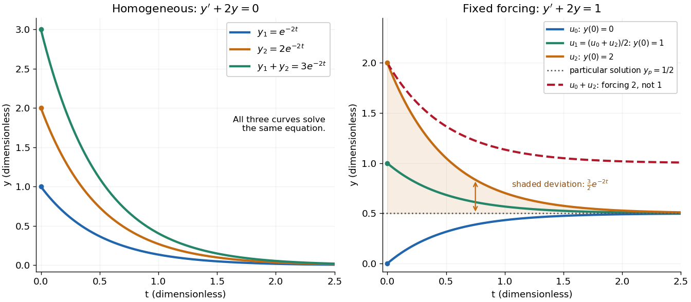
Homogeneous solutions obey superposition, while a fixed forcing term gives a particular solution plus homogeneous solutions
. Details. On the left, all three curves solve the same homogeneous linear differential equation. On the right, share the particular solution , and the shaded difference is the homogeneous solution . The dashed sum has twice the forcing term, even though its starting value coincides with that of . Adding the two initial conditions also adds their inputs; taking their midpoint averages both. This distinction makes the superposition principle useful for assembling responses to different inputs without mistaking that assembly for a solution of a differential equation with the original input. See MIT's superposition notes, including the particular solution one half.
Articles were limited to the first 100 out of 440 total.



