Past exam of the quantum condensed matter course of the University of Cambridge / 2007 / Section A / A3

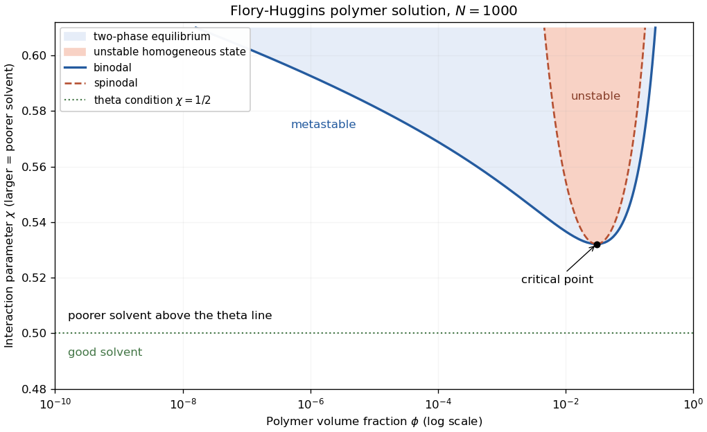
Use polymer volume fraction $\varphi$ and interaction parameter $\chi$, increasing toward poor-solvent conditions. The Flory–Huggins solution theory free energy per lattice site isThe common-tangent construction gives the binodal; $f^{\prime \prime }=0$ gives the spinodal, $2{\chi }_s=1/(N\varphi )+1/(1-\varphi )$. Its critical point is ${\varphi }_c=1/(1+\sqrt{N})$, ${\chi }_c=\frac{1}{2}(1+N^{-1/2}{)}^2$. Above the binodal in this $\chi$ plot, the solution separates into polymer-poor and polymer-rich phases; between binodal and spinodal it is metastable, while inside the spinodal a homogeneous state is unstable.

The line $\chi =1/2$ is the theta solvent condition for a long dilute chain. Below it is the good solvent side; above it is the poor solvent side. Poor solvent does not imply that every composition is already phase separated. Independently, a homogeneous solution is dilute for $\varphi \ll {\varphi }^{\ast }$, semidilute for $\varphi \gg {\varphi }^{\ast }$ below close packing, and concentrated as $\varphi$ approaches one.

Here $R$ denotes a typical chain size, such as an rms end-to-end distance of a polymer chain, rather than the mean end-to-end vector of an isotropic solution, which is zero. The Flory approximation gives $R\sim a{N}^{3/5}$ in a good solvent, an ideal chain has $R\sim a{N}^{1/2}$ in a theta solvent, and a compact polymer globule has size $R\sim a{N}^{1/3}$ in a strongly poor solvent. These are scaling estimates with order-one prefactors omitted, treating the stated $N$ as the segment count associated with the supplied statistical length.

In ethylbenzene, the good solvent makes effective segment repulsions swell the coil. With the Flory approximation,

At the specified theta condition in cyclohexane, the leading effective excluded volume vanishes and the ideal chain estimate is

In water, the strongly poor solvent favours a compact polymer globule. A site-volume estimate givesThe exact numerical conversion between globule radius and rms end-to-end distance depends on its density and shape; this calculation supplies the characteristic size scale.

The polymer overlap concentration corresponds to about one chain per coil volume. Approximating the occupied volume of one statistical segment by $a^3$ givesThus the site-volume model predicts overlap at a few percent volume fraction. A separately specified molecular segment volume or a coil-volume prefactor would change this numerical prefactor.

For a concentration blob with $g$ ideal segments, $\xi \sim a\sqrt{g}$ and concentration matching gives $\varphi \sim g{a}^3/{\xi }^3\sim g^{-1/2}$. Thus the concentration-blob size in a theta solvent isThe whole chain contains about ten blobs, so the separation of scales is moderate. Below $\xi$, theta-solvent segments have ideal chain statistics; above it, screening also gives Gaussian random-walk statistics for the sequence of blobs. There is no good-solvent self-avoiding regime to insert in this particular theta-solvent calculation. Density correlations and segment dynamics can still cross over at the blob scale.

In a dilute solution, solvent-mediated hydrodynamic interactions couple distant chain segments. The Zimm model describes the resulting cooperative dynamics: an intermediate-time segment mean-square displacement scales as $t^{2/3}$, while whole-chain translation has $D_Z\sim k_{B}T/({\eta }_{s}R)$. Once internal modes relax, each tagged segment follows the chain's ordinary long-time diffusion, with mean-square displacement asymptotic to $6D_{Z}t$.

In a concentrated solution or polymer melt, hydrodynamic coupling is screened. The unentangled Rouse model has an intermediate $t^{1/2}$ segment regime and whole-chain diffusivity proportional to $N^{-1}$. Long chains with polymer entanglement are additionally confined by neighbouring chains: reptation gives a slower intermediate $t^{1/4}$ regime and an asymptotic chain diffusivity scaling approximately as $N^{-2}$. The time windows depend on segment, entanglement and terminal relaxation times, so these powers do not all describe the same time interval.

After sufficiently long times both dilute and concentrated chains undergo ordinary translational diffusion. The main long-time difference is the coefficient and its chain-length dependence, with entanglement strongly reducing mobility when the chains are long enough; concentration alone does not guarantee an entangled regime.