The initial table of content was limited to the first level because it is larger than 1000 articles. There are 1870 articles in total. Expand a branch to load its children.
By addition of angular momentum, combining the first two spin one-half particles gives . Adding the third gives the three spin-one-half angular-momentum decompositionThus there is one total-spin sector and two independent sectors. Since the particles are distinguishable, no fermionic exchange symmetry restriction removes either copy. In a simultaneous angular momentum eigenstate, and have eigenvalues and , soThe energy levels and their generic multiplicities areThe count agrees with the dimension of the three-particle tensor product. These multiplicities must be added whenever numerical energy eigenvalues coincide. In particular, for and , there are two fourfold degenerate energy levels, and . For and , the multiplicities at are . If both coefficients vanish, the single energy level has multiplicity eight. Other coincidences between the two total-spin sectors occur when , with from the quartet and from a doublet.
A density matrix has unit trace. The Pauli matrices are traceless, so and hence . Using in the expectation value givesConsequently the required Bloch vector and density matrix areThe two eigenvalues are and , both positive, so this is a valid density operator. Its purity of a density operator isTherefore it is a mixed state. Equivalently, its spectral decomposition is , an ensemble of the two distinct spin one-half along an axis states, rather than a single pure state.
Write the trap angular frequency as and the single-particle oscillator length as . The center of mass coordinate and relative coordinate give independent quantum harmonic oscillators, both of frequency , with masses and reduced mass . Label their excitation numbers by and . The unperturbed energy eigenvalue is .
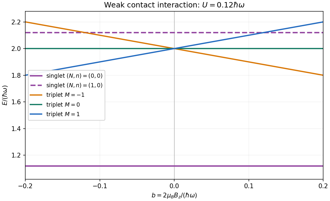
Particle exchange leaves unchanged and sends to . The exchange symmetry of two identical spin-one-half fermions therefore requires even to accompany the spin-one-half singlet state, and odd to accompany a spin-one-half triplet state. For the contact shifts of two spin-one-half fermions in a harmonic trap, the delta potential depends only on . For odd , the relative wavefunction vanishes at , so its contact shift is zero. Within the first-excited manifold, both perturbations are diagonal in the labels : this is a perturbation diagonal within a degenerate eigenspace. For , the relative oscillator length is , giving the first-order nondegenerate perturbation theory shiftThe Zeeman splitting is for total spin projection . Thus the five lowest states, counted with multiplicity, haveunder the assumed conditions . The three triplet states have slopes , while both singlet states are field independent at this order. The three triplet state branches coincide at zero magnetic field. Their crossing with the excited singlet state is allowed because the total-spin sectors do not mix. The odd relative wavefunctions are in fact unaffected by this delta potential at any coupling; the displayed singlet state shifts retain only first order.

Let the electric charge be , where is the elementary charge. Minimal coupling to a tangential magnetic vector potential givesA constant tangential magnetic vector potential is an available gauge on the ring, so . By Stokes theorem, its circulation is the oriented magnetic fluxThe orientation matters here. In the original diagram, increasing goes anticlockwise, whose associated positive normal points out of the page, whereas the indicated positive magnetic flux points into the page. Hence for that diagram, and its convention gives . If instead is defined with the normal associated to , the relation is .
There is no requirement that the magnetic field be nonzero on the ring: it can be confined to a solenoid inside it. The nonzero circulation of the magnetic vector potential still affects the Electron through the Aharonov-Bohm effect.
Define a transformed wavefunction byIndeed, writing givesThis is the electromagnetic gauge transformation generated by : and . The transformed Hamiltonian operator is consequently , but the original periodic boundary condition becomes the twisted boundary conditionFor the domain of the self-adjoint kinetic Hamiltonian operator, the derivative has the same twist, . Thus the magnetic flux has moved into the boundary condition. The transformation is a single-valued gauge on periodic representatives only when is an integer multiple of ; otherwise it is understood on the cut interval with the displayed identification of its endpoints.
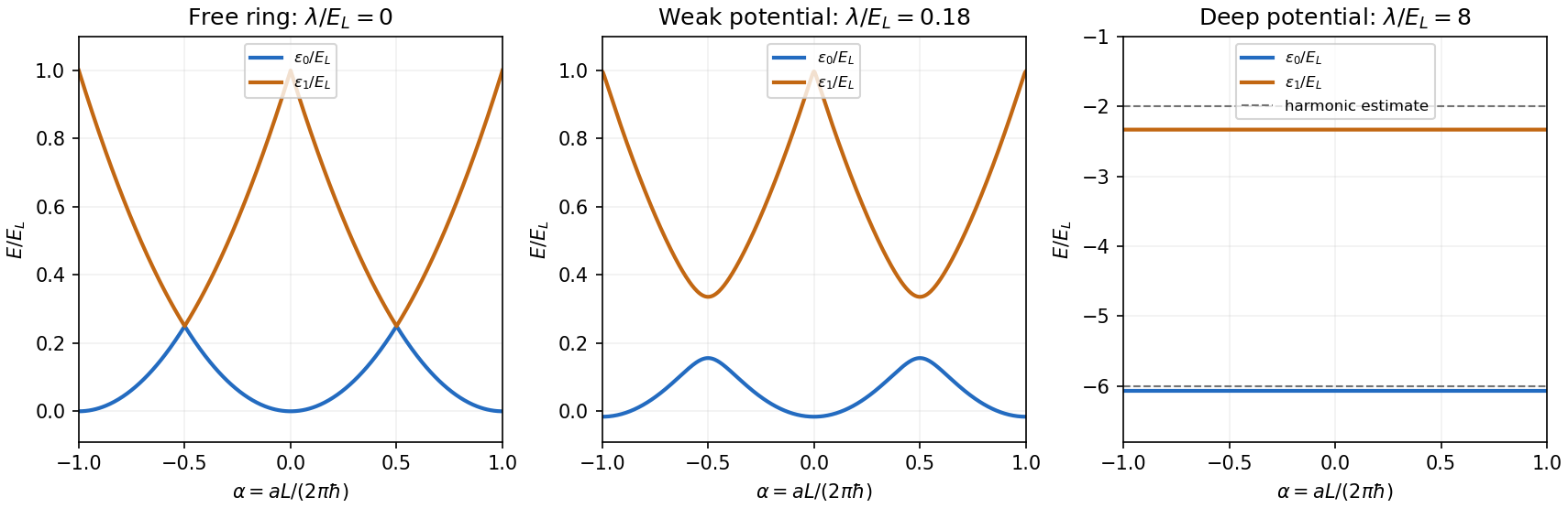
For the magnetic flux spectrum of a quantum ring, the periodic boundary condition permits the normalized plane waves , with . Their energy eigenvalues areShifting by an integer relabels , so the ordered energy levels have period one in , or in . For , the lowest two areextended periodically. The lowest branches cross at every half-integer , with energy . At integer , the first excited energy level has multiplicity two. The corresponding magnetic flux period is the electron magnetic flux quantum .

In the normalized plane wave basis, the only nonzero potential matrix elements areThus a useful small parameter is , which suppresses admixture of well-separated energy levels. First-order nondegenerate perturbation theory further requires for the coupled states. This latter condition fails near a half-integer even for very small ; there one must use degenerate perturbation theory in the nearly degenerate pair. Smallness is measured against the gaps to the other states, not the vanishing gap inside this pair.
Near , keep . The resulting Hamiltonian operator matrix and its eigenvalues areIn particular,For positive , the lower quantum state at the crossing is the symmetric combination of , and the upper state is the antisymmetric combination. A negative exchanges these combinations but leaves the ordered energy eigenvalues unchanged.
This cosine-potential gap in a quantum ring appears in the middle panel above: each lowest-branch crossing opens into an avoided crossing of gap to first order. Away from these crossings, the diagonal matrix elements vanish, so the leading shifts are second order. At integer , the two first-excited plane waves differ by two units of and therefore have no first-order coupling; their smaller splitting begins at second order. The numerical plot includes that splitting.
Put . Changing the sign of translates the potential by without changing its energy eigenvalues, so take a minimum at and expand there. The parabolic approximation givesThe low-lying wavefunctions are localized well inside one period. A local gauge transformation removes from their quantum harmonic oscillator equation, givingConsequently,The sketch consists of two nearly horizontal branches, separated by this gap, as in the right panel above. The parabolic approximation makes them completely independent of magnetic flux; in the actual ring they retain exponentially small periodic dependence through quantum tunnelling around the ring. Corrections from the nonquadratic part of the potential shift the mean energies and gap by relative order , whereas the tunnelling dependence is smaller than every power of that parameter.
The unperturbed infinite square well is invariant under the parity operator. Its one-dimensional energy eigenvalues are nondegenerate, so each energy eigenstate has definite parity. Its position expectation value therefore vanishes: is even, while is odd. The first-order nondegenerate perturbation theory correction is consequentlyThe electric field does mix opposite-parity quantum states, and second-order nondegenerate perturbation theory contains two factors of . Its leading contribution is thus proportional to : this is a quadratic Stark effect. More generally, applying the parity operator changes into , so their corresponding energy eigenvalues agree. An analytic expansion about zero electric field contains only even powers of . We assume is small compared with the unperturbed excitation scale.
Use zero-based labels to agree with in the later parts. The normalized infinite square well energy eigenstates and energy eigenvalues areThe position matrix elements in a symmetric infinite square well, obtained by integrating the product of the two wavefunctions against , areThe integral in the question uses positive integer labels; replacing them by is essential here. Only opposite-parity states, odd, contribute, as also follows from the parity operator selection rule.
Second-order nondegenerate perturbation theory now gives the requested infinite sum:In fully explicit form this isThe symbol here denotes the electron mass, not a summation index. For the ground state , every denominator in the first form is negative, so the ground energy level moves downward. For excited states, contributions from lower and higher energy levels have opposite signs.
The electron's electric dipole moment is . It vanishes in the unperturbed ground energy eigenstate. The first correction to the wavefunction is linear in the electric field and has the opposite parity; its interference with the unperturbed state therefore gives a nonzero position expectation value of first order.
In detail, the normalized ground quantum state, to the order needed, isThe normalization correction starts at second order and does not affect the linear term below. The two cross terms giveThe absence of an term follows from the parity operator: changes sign under field reversal. Comparing with the second-order nondegenerate perturbation theory energy sum yieldsThus the induced electric dipole moment points along the electric field, with positive electric polarizability. The induced dipole moment and quadratic energy shift obey . This factor of one half accounts for the energy needed to induce the dipole. As a check, the Hellmann–Feynman theorem gives , with the same result.
Normalize the trial quantum state as . With the phases used above, the off-diagonal position matrix element is . DefineThe diagonal perturbation matrix elements vanish by parity, so the Rayleigh quotient isThe stationarity equation is . The minimum continuously connected to the unperturbed ground energy eigenstate hasEquivalently, diagonalize the Hamiltonian operator matrix in this two-dimensional trial space. Its lower eigenvalue isThereforeThis retains exactly the term of the full ground-state second-order nondegenerate perturbation theory sum. Every omitted term is negative, so the full quadratic correction is more negative than this restricted one. This is consistent with the Rayleigh-Ritz variational principle: minimizing over a two-state subspace gives an upper bound on the exact ground energy. The bound applies to the unexpanded two-state minimum; a truncated series is to be compared order by order.
For this spin-boson model, take . Since , the interaction picture observable isThe normalized vectors and belong to different eigenspaces of the Hermitian operator , and are therefore orthogonal. This remains true even though each vector includes the oscillator degrees of freedom. Hence all cross terms in the expectation value vanish, while the diagonal terms have eigenvalues and :Normalization also gives , so these are the probabilities of the two spin outcomes.
The orthogonal projection onto the full spin- subspace isHere the identity acts on all oscillator states. The finite-time scattering operator in the question is the interaction picture time-evolution operator, so . Projecting its two orthogonal spin components yieldsExpand the right-hand side in the orthonormal basis . Taking its squared norm, and using the normalization of , givesThus one sums probabilities over unobserved final oscillator states, not their probability amplitudes. Unitarity of makes the sum over both equal to one.
The Pauli matrix flips the spin with unit matrix element. A nonzero oscillator matrix element changes exactly one occupation number, through a creation operator or an annihilation operator:For a spin flip, the spin energy change divided by is . Thus creation and annihilation in mode have total frequency changes and , respectively. Distinct modes or different occupation changes lead to orthogonal final quantum states, so their probabilities add. Fermi's golden rule consequently givesThe Dirac delta function is even, accounting for the sign in the annihilation term. Since all , an initially up spin can only emit an oscillator quantum, while an initially down spin can only absorb one. Writing the oscillator density of states per unit angular frequency as , the continuum limit givesThe permits emission even from the oscillator vacuum; absorption requires a quantum already present. The notation assumes a common or smoothly specified occupation at the resonant frequency. If several resonant modes have different occupations, it denotes their density of states weighted mean, so that after continuum smoothing. This is the golden-rule relaxation of a spin coupled to an oscillator bath.
In first-order time-dependent perturbation theory, the resonant time factor before taking the Fermi's golden rule limit isIts central frequency width is of order , and its total area is . To replace it by , the oscillator density of states and relevant occupations must be approximately constant over that width. Thus . At the same time, the perturbative flip probability must remain much smaller than one.
Define , so the two flip rates are and . A sufficient common time window for both initial spins isFor a specified initial spin, the upper condition is simply its own flip rate times . Such a window requires weak enough coupling. The continuum approximation also presumes times shorter than recurrences from a resolved finite oscillator spectrum, and long enough to resolve the positive-frequency resonance from its nonresonant counterpart.
The thermal oscillator occupation is the Bose-Einstein distribution. With the rate notation for a transition from to , the master equation for the up population isAt thermal equilibrium, assuming , vanishing time derivative is detailed balance between the two spin states. HenceorTogether with normalization, this gives and , the Boltzmann distribution for the energy eigenvalues . At zero temperature, absorption vanishes and emission relaxes the spin into its down ground state.
The nonzero-rate condition is necessary: if or , both rates vanish, so every initial pair of populations is stationary within this approximation. In that case stationarity alone cannot imply a thermal distribution. The equilibrium conclusion therefore presumes coupling to resonant oscillator modes.
The initial quantum state is a coherent state. Since and the state is normalized, its mean occupation number is . Each quantum harmonic oscillator energy eigenstate acquires the phase , soThe prefactor is a global phase and does not change an expectation value. Inverting the definitions of the annihilation operator and creation operator gives . If , thenFor a classical harmonic oscillator with amplitude , the conserved energy is . Setting gives exactly the same amplitude, . Thus these coherent-state oscillator expectation values follow the classical orbit.
The full quantum mean energy is nevertheless : the extra zero-point energy belongs to the nonzero position and momentum uncertainties required by the Heisenberg uncertainty relation, rather than to the motion of the packet centre. In particular, gives zero mean displacement but a finite ground-state width. A coherent state follows a classical mean trajectory while retaining finite position and momentum uncertainties.
Use the uncoupled angular momentum eigenstates and , with . For the Hamiltonian operator actually written in the paper, these are the energy eigenstates, withThe initial states are not all energy eigenstates of this operator. To find their energy populations, first perform the Clebsch-Gordan decomposition. The extremal states are and . Applying the total angular momentum lowering operator to the first givesSimilarly,The initial preparation is an equal incoherent mixture of the four coupled states. Each extremal state contributes population to its one energy eigenvalue, while each nonextremal state contributes and of its own population to the two displayed components. The resulting Zeeman splitting is thereforefor nonzero . The relative populations are in this order; the two zero-energy states each have population . These Zeeman populations from an unpolarized angular-momentum multiplet remain constant under subsequent evolution by the stated static Hamiltonian operator, although off-diagonal quantum coherence can evolve.
There is a distinct weak-field model in which a retained spin-orbit interaction keeps isolated and one projects the magnetic perturbation into that quartet. The Landé g-factor is then , giving four shifts with equal populations. That calculation requires the additional projection or dominant spin-orbit interaction; it is not diagonalization of the full magnetic Hamiltonian operator specified here, which also mixes the sector.
A confined ground state requires ; take so the trial wavefunction is normalizable. Its normalized form isThe Gaussian moment recurrence gives and . Also, integration by parts gives . The Rayleigh quotient for the quartic oscillator is consequentlyDifferentiation yields , so the unique minimum is at . Since the quotient diverges at both endpoints and , this is the global minimum in the trial family. The Rayleigh-Ritz variational principle givesFor the first excited energy eigenstate, choose the odd trial familyThe even confining potential has an even, nodeless ground state, by the nodeless theorem for a one-dimensional ground state. By the Sturm oscillation theorem, its first excited state is odd with one node. The proposed family has the same parity operator eigenvalue and one node, and is orthogonal to the exact ground state, not merely to its Gaussian trial approximation. Minimization in the odd linear subspace therefore bounds the first excited energy from above. For completeness, its Rayleigh quotient is , minimized at , giving . These are Gaussian variational bounds for a quartic oscillator.
If , there is no normalizable free particle ground state on the whole line, though the spectral infimum is zero. If , the Hamiltonian operator is not bounded below, so a ground-energy bound of the requested kind does not exist.
Start with the Schrödinger equation and differentiate the definition of the interaction picture state:The free Hamiltonian operator terms cancel because commutes with its own matrix exponential. ThereforeThis interaction picture transformation is exact.
Write and use the ordered spin basis . The free Hamiltonian operator is , soResolving the cosine into its two complex exponentials gives the exact upper off-diagonal factorwith the complex conjugate in the lower entry. Choose the field orientation with , as implicit in the printed near-resonance condition, and put . The rotating-wave approximation discards the terms at , retaining the slow terms at . The resulting interaction picture equations areThe factor contains from and from the cosine decomposition. This is a Driven two-level Rabi model, with signed on-resonance coupling and generalized Rabi angular frequency . Here the Rabi detuning uses the paper's convention, drive minus free frequency.
Small detuning alone is insufficient to derive the printed equations. One also requires , and an evolution time over which neglected terms stay small. At resonance this is the weak transverse-field regime . The supplied solution is thus an approximate solution for the linearly oscillating field, not an exact one at arbitrary drive strength. If , the other exponential is resonant and the physical positive resonance frequency is .
With , the Born rule applied to the supplied down-spin probability amplitude givesFor nonzero transverse field, the maxima occur atThe first maximum is reached at ; on resonance this is a Rabi pi pulse. The resonance envelope of a Rabi transition is a Lorentzian line shape, centred on under the orientation convention above. It has half its peak value at , so its full width at half maximum isIf resonance width is instead defined as the half-width, the ratio differs by a factor of two but has the same requested proportionality. The quality factor is large precisely in the regime where the rotating-wave approximation is justified. The envelope is obtained by choosing the best time separately at each drive frequency; a measurement at one fixed pulse duration has a different line profile.
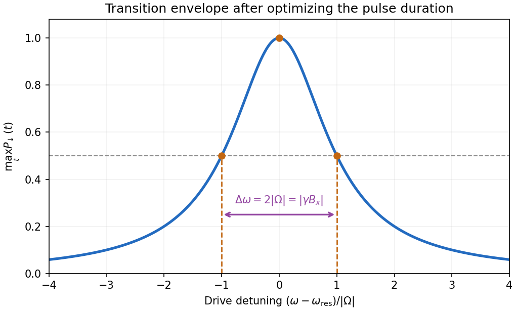
Maximum spin-flip probability versus drive detuning
. Original rotating-wave approximation envelope, with the two half-height detunings marked. The maximum is over interaction time independently at each drive frequency. Details.
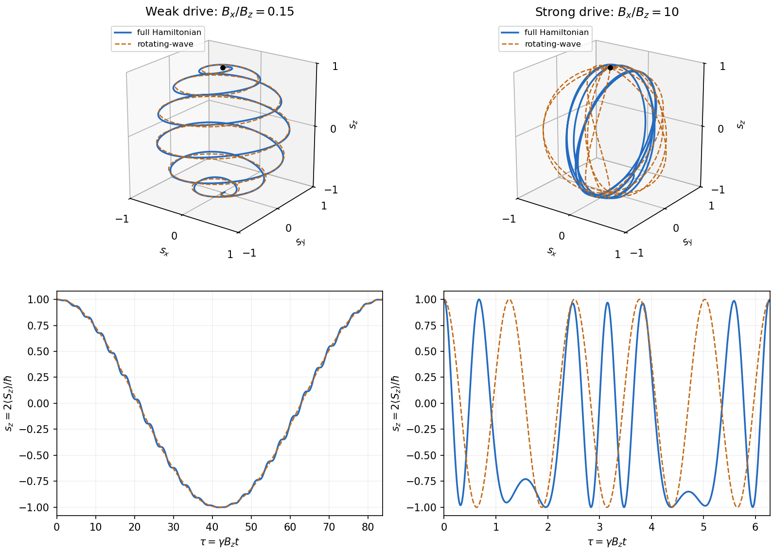
At resonance, retain the signed coupling . In the interaction picture, the given solution reduces to and . Returning to the Schrödinger picture givesFor a normalized spinor , the Pauli matrices give . Therefore the spin expectation value within the rotating-wave approximation isIts magnitude is : the Bloch vector stays on the unit sphere. In a frame rotating about at angular velocity , it makes a uniform rotation in the plane. For , this gives slow Rabi oscillations between the poles, accompanied by rapid laboratory Larmor precession about .
If the same formula is formally used for , it predicts fast meridional rotations whose plane turns slowly about . However, the original PDF really does ask for this opposite limit, and it lies outside the assumption used in part (b). That formal description is not a controlled prediction for the stated linearly driven Hamiltonian operator.
A valid strong-drive description starts from the exact equation for the Bloch vector :For times , neglecting the weak bias gives a controlled leading approximation, since the time integral of the omitted Hamiltonian operator has small norm. The remaining field has a fixed axis, so its generators commute at different times andAt the nominal resonance and on the early spin-rotation scale , this becomes . The initial rotation rate is consequently , twice the rate predicted by extrapolating the rotating-wave approximation. For longer times the exact differential equation must be retained. The following original calculation illustrates both regimes rather than asserting an exact strong-drive Rabi formula.

The components of the momentum operator do not generally commute with a position-dependent magnetic vector potential. Expanding minimal coupling with the ordering intact givesActing on a wavefunction shows that . In the Coulomb gauge the divergence vanishes, so the two cross terms agree. Discarding the quadratic term in the weak radiation amplitude givesThe equality of the two operator orderings follows from the gauge condition, not from treating and as commuting numbers component by component.
For the requested oscillator response, treat as the fixed transverse position of a one-dimensional quantum harmonic oscillator along , and put . The supplied radiation is transverse and already satisfies the Coulomb gauge. Its perturbation isThe annihilation operator and creation operator giveThus the only first-order transition out of the ground state is to . More generally, the oscillator electric-dipole selection rule is . This is a rule for matrix elements; exact energy conservation is replaced by a finite-time resonance profile during a switched finite-duration interaction.
To display both the resonant and nonresonant terms without spurious singularities, defineThe interaction picture coefficient in the given expansion is thenThe full Schrödinger picture coefficient of is , while that of is at this order. The normalization changes only at order . In particular, at the first term is , finite for every finite time, and the perturbative result requires .
The fixed- interpretation is needed for the displayed target formulae. If were instead a three-dimensional kinetic operator with no transverse confinement, that model would have no normalizable transverse ground state, and would transfer transverse momentum . A treatment of that different model needs specified transverse states and recoil energies; they are absent from the question. The following parts use the intended localized-oscillator response.
The only relevant position matrix element is . To first order in the radiation amplitude, the two ground–excited-state cross terms giveMultiplying by the charge gives the induced electric dipole moment. Since , the coefficient derived in part (b) yieldsat linear order. Taking the complex conjugate inside the real part of the second term changes it to minus the same term with and reversed frequency signs. ThusThe terms at are switch-on transients, while those at describe the driven response. Both are needed to make . The expression is understood by continuity at ; the first quotient then tends to , producing resonant secular growth rather than an infinite dipole at a finite time.
There is also an initial-velocity check on this harmonic-oscillator dipole response to switched radiation. The formula gives . Because the magnetic vector potential jumps at zero time, its time derivative contains an impulsive electric field. Equivalently, the mechanical velocity is , whose initial mean is . The transient therefore implements the specified switch-on correctly.
For , isolate the terms proportional to in the previous answer. Their coefficient isHence the driven electric dipole moment component isFor , away from the instantaneous switch, the radiation electric field isThus the dynamic electric polarizability isBelow resonance the driven electric dipole moment is in phase with the electric field; above resonance its sign reverses. The same susceptibility follows from the classical Lorentz oscillator model without damping. At exact resonance the separation into bounded driven and transient terms fails: their apparent poles combine into the finite-time secular term identified in part (c). Without damping there is no bounded steady resonant response, and the first-order state expansion eventually ceases to apply.
Inside the infinite square well, the orbital and spin operators act on different factors of the tensor product. Write . The identityshows that the exchange interaction commutes with and . The sum of the one-particle kinetic energies also commutes with them and with particle exchange. Thus one may use orbital quantum numbers together with the total-spin sector and projection , with physical .
For identical spin one-half particles the Pauli exclusion principle further restricts the states. The spin-one-half singlet state is antisymmetric in spin and must multiply a symmetric spatial wavefunction; a spin-one-half triplet state must multiply an antisymmetric spatial wavefunction. Thus label unordered orbital occupations in symmetry-adapted states, not arbitrary ordered product states. This gives the labels , with the paper's last label expressed in units of .
LetThe normalized orbital energy eigenstates vanish outside the well and have one-particle energies . Define the normalized symmetric and antisymmetric combinations for byThe normalized spin functions are the singlet state and the triplet states , , . Their exchange energies are respectively and .
For , the three lowest distinct energy levels of the exchange-coupled spin-one-half particles in an infinite square well areThe spatially doubly occupied orbital can only occur with the singlet state. The next orbital sum is , where either exchange symmetry is possible. The next unused sum is , well separated under the small-coupling assumption. The paper's inequality is equivalent, up to a numerical factor, to ; the factor in is essential because the spin operators carry units of angular momentum.
The sign of is not explicitly specified. The table assumes the usual intended positive coupling in the displayed minus-sign convention. For with , the same three sets of eigenfunctions occur, but the two rows at exchange order. At those rows merge into a single energy level of multiplicity four; if three distinct energies are requested exactly at that point, the third is with the single state .
Each one-particle energy eigenstate has definite parity about the centre of the well, so . Consequently, a doubly occupied orbital has . For distinct orbitals, the two off-diagonal exchange terms instead survive:The position matrix elements in a symmetric infinite square well, with the present width , giveThe sign of depends on the orbital phase convention, while does not. The perturbation acts only on the spatial part and cannot mix orthogonal singlet states and triplet states. Within a triplet it is proportional to the identity on the spin factor. Thus first-order nondegenerate perturbation theory, with this trivial diagonal treatment of spin degeneracy, gives the shifts corresponding to the three rows in part (b):These formulae also apply for , with the reordered levels described above. At , they resolve the fourfold level into a shifted triplet and singlet. The next doubly occupied orbital still has zero first-order shift. The perturbative requirement is for mixing with remote orbital states; the spin-independent perturbation does not require division by the small singlet–triplet gap.
For distinguishable particles, the ordered spatial products are independent states, and neither singlet states nor triplet states are excluded from any orbital occupation. The unperturbed energy eigenvalues areFor , the three lowest distinct energy levels arewhere . The first two levels do have zero first-order correction, since their spatial expectation value factorizes as .
The last instruction in the original PDF is false for the third level. Although every diagonal product-state matrix element vanishes, the two orbital states have degenerate energy levels. Degenerate perturbation theory requires diagonalizing the perturbation within their span. For each , its matrix in the ordered basis isThe eigenfunctions are , withThus the sixfold unperturbed level splits into two triplets. Its average shift is zero, and the diagonal expectation in an individual ordered product state is zero, but neither fact makes all its energy eigenvalue corrections zero. This is the degenerate orbital exchange splitting from a product perturbation; distinguishability allows both combinations rather than removing their coupling.
For negative , the lowest two rows exchange order and the third unperturbed level is instead the twofold singlet orbital pair at . It splits into with the same shifts , each nondegenerate. At , the three lowest distinct unperturbed energies are , with multiplicities . The first and third have zero first-order shift; the middle splits by , each fourfold. The printed zero-shift assertion therefore fails also in the zero-exchange limit.
The closed and subshells contribute zero total orbital angular momentum and spin, so only the two electrons matter. The first of Hund's rules maximizes their total spin, giving . The Pauli exclusion principle then requires an antisymmetric spatial wavefunction. Two parallel-spin electrons cannot occupy the same orbital: the greatest possible orbital projection is , so the maximal allowed within this triplet is .
The ground term is therefore , in term symbol notation . Since the subshell contains fewer than half of its six possible electrons, the third of Hund's rules places the smallest lowest. Addition of angular momentum gives , in that energy order within the ground term. ThusThese are the fine structure partners of the same electronic term, with magnetic multiplicities , rather than different principal-shell excitations. The ordering agrees with the tabulated lowest neutral-carbon levels.[ref]
https://physics.nist.gov/PhysRefData/Handbook/Tables/carbontable5.htm. NIST, Energy Levels of Neutral Carbon, lowest three entries
Let be the spontaneous emission coefficient, and let and be the absorption and stimulated emission rates per atom under the radiation spectral energy density at resonance. Because the two levels are nondegenerate, the Einstein coefficients satisfy .
The radiative balance in a nondegenerate two-level atom isThe total spontaneous and stimulated emission rates are and . Dividing the balance equation by givesThis presumes nonzero drive and upper-level population, and no other population-transfer mechanism. It does not require a thermal Boltzmann distribution. In this closed driven two-level system, spontaneous decay keeps ; arbitrarily intense driving approaches equal populations, rather than producing a population inversion.
Use the electronic weak-field Zeeman splitting model, neglecting hyperfine structure. The Landé g-factor is for and for . The shift of an absorption frequency is thereforeHere the magnetic field is weak relative to spin-orbit coupling, so remains a useful quantum number, but the spectral line widths are small enough to resolve its magnetic substates.
For linear polarization parallel to , the optical electric field has only the field-axis component. The electric-dipole selection rule is . Its two allowed transitions are , givingFor propagation perpendicular to with linear polarization also perpendicular to , the optical electric field is an equal-amplitude combination of the two field-axis circular components. It drives transitions with . These connect and , givingThus each orientation selects two lines, with twice the separation in the perpendicular-polarization case. Neither pair has an unshifted central component. This is polarization-selective Zeeman splitting of an alkali D1 line, an anomalous Zeeman effect rather than a normal orbital triplet.
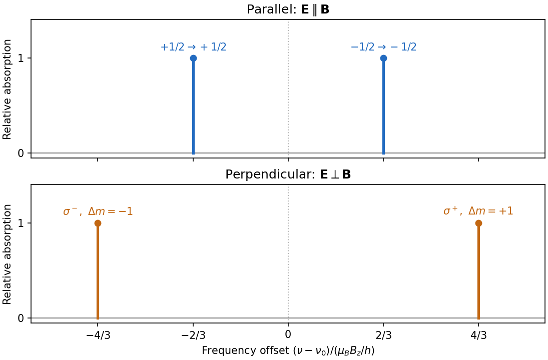
Polarization selects two different sodium D1 Zeeman doublets
. Original electronic-level prediction in units . Equal heights within each pair illustrate an initially unpolarized lower level and a weak probe; optical pumping can alter populations and hence strengths. Hyperfine structure is omitted, as in the stated electronic -level model. Details.
For a self-adjoint Hamiltonian operator bounded below with ground-state energy , every admissible nonzero trial wavefunction has a Rayleigh quotient at least . To see this explicitly in a complete orthonormal eigenbasis, write with . ThensoFor continuous spectral components, the spectral theorem replaces the sum by an integral with the same nonnegative integrand. Equality requires the trial quantum state to lie entirely in the ground-state subspace. The variational method chooses a tractable family, evaluates the quotient and minimizes over its parameters. This gives an upper bound; enlarging the family can only improve that bound. The trial must belong to the operator domain for the operator expression above, or have finite energy in the corresponding quadratic-form version of the quantum variational principle.
For the oscillator, use the standard kinetic operator : the original PDF omits the superscript on the derivative in its numerator. Take , and normalize the scaled exact ground state asThe factor is optional in a quotient but makes the calculation transparent. Changing variable to and differentiating the scaled wavefunction givesAt this trial is the exact minimizing state, so its energy has zero derivative there. Hence . Since ,This is the quantum virial identity from scaling for a quadratic potential, and hence the oscillator form of the virial theorem.
For the inverse-power attraction, take and suppose, for contradiction, that an exact ground state exists with separately finite kinetic energy and potential mean , admitting the same dilation variations. Homogeneity now givesStationarity at would require . Its second derivative would then beFor this is negative, contradicting a ground-state minimum. More strongly, one does not need a presumed exact state: choose any normalized smooth test function supported away from the singular origin. Its and are finite, and its scaled quotient satisfiesThe unregularized attraction therefore exhibits fall to the centre for a supercritical inverse-power potential and has no stable ground state.
There is a necessary qualification to the PDF's broader wording about “no bound state”. Under the usual finite-energy virial theorem assumptions, a putative negative-energy bound state would satisfywhich contradicts being below the continuum threshold at zero. Thus no negative-energy bound state satisfying those regularity assumptions is possible. But this singular differential expression needs a specified domain at ; separately divergent kinetic and potential means or boundary conditions not preserved by dilation invalidate that ordinary calculation. The domain assumptions in singular-potential virial arguments must therefore be stated: the scaling proof establishes absence of a semibounded ground-state problem, rather than a domain-independent theorem about every formal square-integrable solution. A short-distance regularization would be a different potential.
The single-electron isotropic quantum harmonic oscillator has energiesIts lowest spatial orbital, denoted , is unique, with energy . Including spin one-half gives two spin orbitals. Two identical Electrons can occupy both only with opposite spin in the unique singlet state. Thus the two-electron ground state has energy and multiplicity one.
The first excited spatial shell consists of , each of energy , giving six spin orbitals. A first-excited two-electron Slater determinant occupies one of the two ground-shell spin orbitals and one of these six excited-shell spin orbitals. HenceNo further factor of two is inserted for interchanging the electrons, since the fermionic exchange symmetry is already built into a Slater determinant.
The spatial Hamiltonian operator is invariant under simultaneous rotations of both positions, so for each component of the total orbital angular momentum. It is also spin independent, so for each total spin component. Thereforeexpressing conservation of angular momentum and conservation of the total spin magnitude for this model. The Pauli exclusion principle restricts which states occur but does not break either symmetry.
To change the first-shell basis, take normalized real Cartesian orbitals . Using spherical coordinates, and . Comparison with the spherical harmonics gives the Cartesian and spherical bases of the first oscillator shell:Each is a common radial factor times , so and . Their normalizations and mutual orthogonality follow because this is a unitary change of basis. The ground spatial orbital has .
For two ground-shell electrons, addition of angular momentum gives , and their symmetric spatial state requires . For one electron in each shell, gives only . For each , form the normalized spatial combinationsThe exchange symmetry of two identical spin-one-half fermions permits with the singlet state and with each triplet state . In term symbol notation the manifolds are thereforeThe count reproduces and , as required. Both exchange symmetries are possible for the distinct occupied orbitals; dropping either spin sector would undercount the two-electron states in the first two shells of an isotropic oscillator.
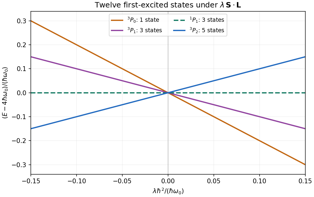
For the specified spin-orbit interaction, and are the total two-electron operators. Set . The spin-dot-product eigenvalue identity givesFor the singlet, and the shift is zero. For the triplet, . The spin-orbit splitting of the first excited two-electron oscillator level is consequentlyAdd each shift to . The multiplicities sum to twelve and their weighted shift sums to zero. For positive the table is ordered in energy; for negative the ordering reverses. Weak coupling means . Since this total-spin interaction commutes with , and , the shifts within this invariant manifold are in fact exact for the specified model, although only first order was requested.

Expand the time-dependent quantum state in unperturbed energy eigenstates, factoring out free dynamical phases:The Schrödinger equation gives the exact interaction picture coefficient equationsInitially . To first order in time-dependent perturbation theory, replace the coefficients on the right by these zeroth-order values and integrate. ThusFor a transition , this is the desired leading probability amplitude, and to leading order. The formula is understood with free asymptotic phases removed. For , the full survival amplitude also contains the zeroth-order ; the displayed integral alone is its first-order correction, not the whole amplitude. This specifies the usual scattering operator meaning of the paper's notation at infinite times.
For the ion pulse, write and . ThenConsider an excitation with and put , . The first real pulse is even in time and the second is odd. Their respective surviving Fourier components are therefore cosine and imaginary sine:Since , the longitudinal term is smaller for comparable position matrix elements. Hence the electric-dipole excitation by a passing ion hasThis leading limit extends to either sign of using . If by a selection rule, the retained leading term vanishes and the smaller longitudinal term may give the first nonzero probability. The conditions also include a small total transition probability, approximately straight constant-velocity motion, and large compared with atomic size for the electric-dipole approximation. The paper uses a Coulomb-coupling convention in which the factor is written ; in SI units replace throughout by .
The collision duration is of order . Excitations with angular frequency receive an unsuppressed impulse when this is short relative to . In contrast, for , cancellations in the Fourier transform suppress the transition: a slowly varying distant field approximately preserves the atomic energy eigenstate. The exact dipole-pulse transforms make this explicit:where is a Modified Bessel function of the second kind. Their large-argument exponential decrease explains the slow-passage cutoff. These transforms are optional refinements of the small- derivation above, not a separate assumption about the target.
To connect the microscopic transition probability to energy loss, suppose the atom begins in a low-energy state. Exciting bound electronic states and causing ionization transfer positive energies from the ion to the material. For target atomic number density and path length , a schematic independent-encounter sum iswith a continuum integral as well as a sum for ionized final states. The short-collision formula gives , so the impact-parameter integral has logarithmic dependence on its cutoffs. Its upper effective cutoff is of order , where the transition ceases to be sudden; the lower cutoff must exclude regions where the dipole or weak-collision approximation fails. Thus the leading high-speed charge and isotope scaling of electronic stopping isAlthough a faster ion can access more energetic transitions and a wider range of distant encounters, its shorter interaction time reduces each ordinary excitation probability. In the fast-ion regime shown, the decrease dominates the slower variation of the excitation factor. The energy loss consequently falls with increasing incident kinetic energy. The original figure has increasing downward, so the curves' rise toward the top of the page means decreasing loss, not increasing loss. A low-speed extrapolation of the inverse-square law is invalid because excitation thresholds, slow-passage suppression, changing ion charge and nuclear recoil can then matter.
For nonrelativistic ion mass , . At fixed incident energy the leading prediction becomesThe greater atomic number of nitrogen than carbon than boron therefore gives larger loss; at the same velocity the leading species factor is . Within an isotopic family, the heavier ion moves more slowly at the same and loses more energy. Equivalently, a heavier isotope needs proportionally greater kinetic energy to achieve the same velocity and approximately the same electronic loss. Comparing at fixed energy per nucleon, rather than fixed total , approximately removes this leading isotope mass dependence. This accounts for the separate isotope bands in the original graph without assigning different electronic excitation spectra to isotopes of the same projectile element.
The charge in this scaling is the effective ion charge if screening by bound projectile electrons is important. The interpretation assumes the same traversed material and thickness and uses the paper's small-fractional-loss regime, ; points with loss comparable to incident energy cannot be described quantitatively by treating as constant. The plotted curves support the qualitative ordering and high-energy decrease, rather than determining a universal normalization from the supplied single-atom model.
Use for a product of the two individual spin-one spin eigenstates, with magnetic quantum numbers . Total requires , leaving preciselyHere these are product labels, not labels of the total angular momentum. Write their coefficients in this order as . With physical spin ladder operators , each nonzero individual step has amplitude , soBoth must vanish for a singlet state. The independent product states therefore require . Wavefunction normalization gives the spin-one singlet stateup to an overall quantum phase. Conversely, implies through , so these conditions really select total spin zero. Distinguishability imposes no additional exchange restriction. The ladder hint uses dimensionless angular momentum units; restoring its common factor does not change the coefficient ratios.
Articles were limited to the first 100 out of 1870 total.
Articles by others on the same topic
There are currently no matching articles.