Past exam of the short options paper shared by Prelims and Parts A and B of the physics course of the University of Oxford / 2015 / S25 / 2 / 2

Take the logarithmic forcing law with its normalization fixed by the given doubling value. Let $x$ be the positive magnitude of cooling and $f$ the positive magnitude of the earlier negative forcing:At $C=212\mathrm{ppm}$, $f_0=1.5051\mathrm{W}{\mathrm{m}}^{-2}$. Equilibrium then yieldsThe concentration endpoints $185$ and $244\mathrm{ppm}$ imply forcing magnitudes $2.242$ and $0.7445\mathrm{W}{\mathrm{m}}^{-2}$, approximately $f_0\pm 0.75$. Define normalized variables $u=f/f_0$ and $v=x/x_0$. 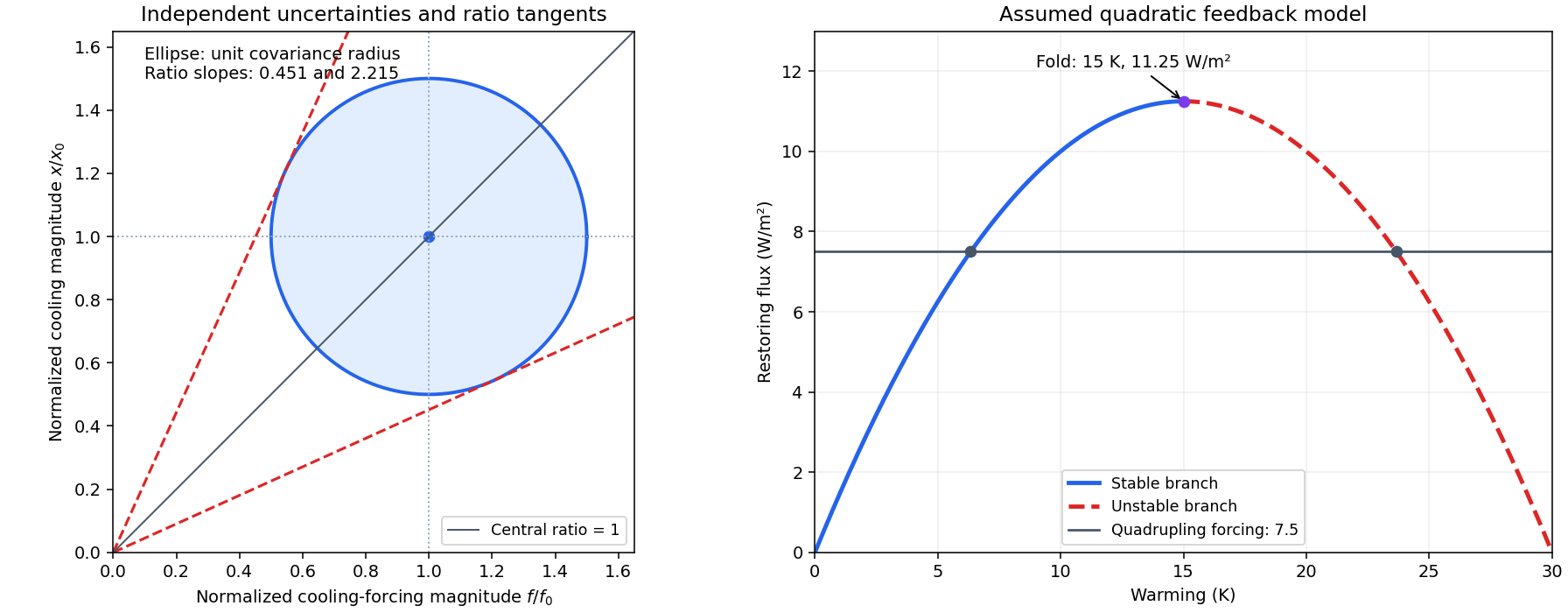Independent approximately Gaussian uncertainties give the one-standard-deviation covariance ellipseIts centre is $(1,1)$ and its principal directions are the two coordinate axes. Warming is $2.492(v/u)\mathrm{K}$, so rays from the origin have constant inferred warming. The bounding rays tangent to this ellipse have slopes $m$ satisfying $(1-m{)}^2=\frac{1}{4}(1+m^2)$, orThis gives the useful asymmetric one-parameter profile estimateThe concentration data supply only marginal intervals, not a full likelihood. This result explicitly approximates their logarithmic forcing uncertainty as Gaussian. Linear error propagation would instead give fractional uncertainty $\sqrt{0.5^2+0.5^2}=0.707$, or roughly $2.49\pm 1.76\mathrm{K}$, and misses the large reciprocal asymmetry. A unit-radius two-dimensional covariance ellipse itself contains about $39\%$ of a bivariate Gaussian, not $68\%$; the quoted interval uses the one-parameter $\Delta {\chi }^2=1$ profile/ratio construction, rather than claiming that ellipse is a $68\%$ joint region.