Past exam of the short options paper shared by Prelims and Parts A and B of the physics course of the University of Oxford / 2015 (A14119W1/A14140W1)

Source paper: www.whatdotheyknow.com/request/physics_preliminary_past_papers/response/2680788/attach/2/2014%202017%20Physics%20Prelim.zip?cookie_passthrough=1

Unlettered marked requests are numbered in source order; explicit letters and Roman parts are retained. S18 worked notes are linked below; their missing amplitude sketch is supplemented here.

Choose the principal logarithm, so $L(z)=\mathrm{Log}(1-z)$ has branch cut $[1,\infty )$. Near zero its Taylor series givesThus zero is a simple pole of residue one, and one is a logarithmic branch point. The function is holomorphic on $\mathbb{C}\setminus (\{0\}\cup [1,\infty ))$ with this branch. Infinity is also a branch point in the extended-plane description; the function's decay there along the cut plane does not make it a single-valued holomorphic function through infinity.

Use the positive orientation shown in the source: the upper bank runs outwards and the lower bank returns towards one. On those banks the logarithm branch has values $\ell -i\pi$ and $\ell +i\pi$, respectively, with $\ell =\log (x-1)$. Their squared difference is $-4i\pi \ell$. The residue theorem therefore givesand henceThe large-circle contribution is $O(R^{-2}{\log }^{2}R)$ and the small circle about one contributes $O(\epsilon |\log \epsilon {|}^2)$, both tending to zero. These estimates justify replacing the closed contour integral by its two cut-bank integrals.

Take $g(z)=L(z{)}^3/z^3$ on the same logarithm branch. At zero, $L(z{)}^3=-z^3+O(z^4)$, so the apparent singularity is removable and the closed contour integral is zero. The bank difference isThe circular contributions vanish by the previous estimates with the third power of the logarithm. ConsequentlyThe last integral is $1/2$, givingIncreasing the logarithm power has converted the desired real integral into a jump across a branch cut, while removing the pole inside the contour.

A conformal map preserves the magnitude and orientation of angles between intersecting smooth curves locally. For a complex holomorphic function, the condition at $z_0$ is $f^{\prime }(z_0)\ne 0$: the first-order change $\delta w=f^{\prime }(z_0)\delta z$ rotates and uniformly scales every tangent vector by the same complex factor. This local statement does not require a globally one-to-one map.

No region maps onto the entire finite complex plane: $e^z$ is never zero. Its image on $\mathbb{C}$ is $\mathbb{C}\setminus \{0\}$. A fundamental strip such asmaps bijectively onto that punctured plane, because $e^{x+iy}=e^x{e}^{iy}$. The half-open strip supplies one representative of each angle; it is not an open domain. An open strip of height $2\pi$ omits a ray as well. The missing zero is approached only in the limit $x\to -\infty$.

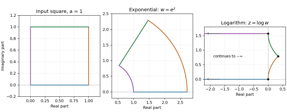
Writing $z=x+iy$ gives $|w|=e^x$ and $\arg w=y$. Thus the closed square maps to the annular sectorIts horizontal edges become radial segments and its vertical edges become circular arcs. Each radial tangent is perpendicular to the tangent of its adjoining circle, so the four interior angles remain $\pi /2$. Equivalently, the complex derivative $e^z$ is nonzero at every vertex and the map is conformal there.

Use the complex logarithm with $0\le \arg w\le \pi /2$ on the nonzero points of the first-quadrant square. Put $z=x+iy=\log |w|+i\arg w$. The square bounds $\mathrm{Re}w,\mathrm{Im}w\le a$ giveThe two edges meeting at $w=0$ map to the horizontal half-lines $y=0$ and $y=\pi /2$, extending indefinitely to the left. The other edges map to $x=\log a-\log \cos y$ for $0\le y\le \pi /4$ and $x=\log a-\log \sin y$ for $\pi /4\le y\le \pi /2$. They meet at $\log (a\sqrt{2})+i\pi /4$.

The angles are preserved at $a$, $a(1+i)$ and $ia$. There $d\log w/dw=1/w$ is finite and nonzero. The origin is a branch point, has no finite logarithmic image, and supplies no fourth finite vertex at which angle preservation could be asserted.

For $t>0$, close the real-axis contour in the upper half-plane: $|e^{izt}|=e^{-t\mathrm{Im}z}$ supplies decay. The only enclosed simple pole is $z=i$, with residue $e^{-t}/(2i)$. Thus $h(t)=2\pi i{e}^{-t}/(2i)=\pi e^{-t}$.

For $t<0$, close downwards. The clockwise orientation contributes $-2\pi i$ times the residue $e^t/(-2i)$ at $z=-i$, givingAt $t=0$, direct integration of $1/(1+p^2)$ gives $\pi$, consistent with the continuous extension. The large arc tends to zero by Jordan's lemma for nonzero $t$, or the denominator estimate when $t=0$.

Let $I$ denote the requested integral. Symmetry and the period of ${\sin }^2\theta$ make the corresponding integral over $0\le \theta \le 2\pi$ equal to $4I$. With $z=e^{i\theta }$, this becomesThe denominator factors as $-2(z^2-1/2)(z^2-2)$. The two poles inside the unit circle are $z=\pm 1/\sqrt{2}$. Each residue is $1/(6i)$, because the derivative of the polynomial denominator there is $6z$. The residue theorem gives $4I=2\pi /3$, so

For the two-body problem, the centre of mass lies a distance $a{M}_J/(M_{\odot }+M_J)=a/1048$ from the Sun. With $a=5.2\mathrm{AU}$,The relative circular-orbit period is $P=2\pi \sqrt{a^3/[G(M_{\odot }+M_J)]}\simeq 11.85$ years. The Sun's orbital speed about that centre of mass is thereforeThis is the space-speed amplitude; the observed radial velocity amplitude also includes the orbital inclination.

Kepler's third law is $P^2=4{\pi }^2{a}^3/[G(M_S+M_P)]$, with $a$ the semimajor axis of the relative orbit. For a circular edge-on orbit, the star's speed is $V_S=2\pi a_S/P$, and the centre of mass relation gives $a_S=a{M}_P/(M_S+M_P)$. Cubing the speed expression and eliminating $a$ yieldsFor $M_P\ll M_S$, this reduces toWithout the edge-on assumption, a factor ${\sin }^{3}i$ multiplies the numerator, explaining the minimum-mass degeneracy of the radial-velocity method.

Converting luminosity to mass needs a main-sequence mass-luminosity relation. Using the near-solar approximation $L/L_{\odot }\simeq (M/M_{\odot }{)}^4$ gives $M_S\simeq 0.946M_{\odot }$. ThenFor $P=11.6$ days and $V_S=10\mathrm{m}{\mathrm{s}}^{-1}$, these give approximatelyThese estimates retain the circular, edge-on and low-companion-mass assumptions. Adopting a mass-luminosity exponent $3.5$ instead changes the quoted values by about one percent; luminosity alone does not determine a unique stellar mass without such a calibration.

The effective temperature is defined by the Stefan–Boltzmann law applied to a star's total luminosity:Here $R$ is the adopted photospheric radius and ${\sigma }_{\mathrm{SB}}$ is the Stefan-Boltzmann constant. This defines the temperature of a black body radiating the same total flux per unit surface area; it does not assert that every wavelength of the stellar spectrum follows a perfect Planck spectrum.

The parallax gives $d=1/0.00763\simeq 131\mathrm{pc}$. Ignoring extinction, the distance modulus givesThe bolometric magnitude relation then yields $L/L_{\odot }=10^{0.4(4.72-M_{\mathrm{bol}})}\simeq 2.53\times 10^4$. With $T_{\odot }\simeq 5772\mathrm{K}$,A star this cool and luminous belongs to the red-supergiant region of the Hertzsprung-Russell diagram. Extinction and the adopted effective temperature are important systematic inputs; this calculation uses the supplied temperature to infer the radius.

A first distance-independent method fits the continuum shape or a calibrated colour index to an atmosphere model. A black-body approximation uses Wien's displacement law, ${\lambda }_{\max }T\simeq 2.90\times 10^{-3}\mathrm{m}\mathrm{K}$, or ratios of the Planck spectrum at two wavelengths. It requires a known extinction correction and sufficient treatment of molecular absorption and line blanketing; a cool supergiant need not have a black-body colour temperature equal to its effective temperature.

A second method fits temperature-sensitive spectral lines or molecular bands. Boltzmann excitation and the Saha equation explain why excitation and ionization ratios change with temperature; detailed atmosphere calculations also include surface gravity, composition and departures from local thermodynamic equilibrium. TiO molecular bands are particularly useful for cool stars. Line ratios remove the overall distance normalization, but their calibration remains model dependent.

The direct flux-radius method can be made distance independent as well: an independently measured angular diameter $\Theta$ gives $T_{\mathrm{eff}}=[4F_{\mathrm{bol}}/({\sigma }_{\mathrm{SB}}{\Theta }^2){]}^{1/4}$. For a large nearby supergiant with a resolved photosphere, good bolometric flux and a limb-darkened interferometric angular diameter, this is often the most direct determination. Its advantage depends on those measurement uncertainties and a consistent radius definition. The radius inferred in the preceding part cannot itself provide an independent temperature measurement, because the supplied temperature was already used to calculate it.

The virial theorem for a stationary isolated system with inverse-square gravity iswhere $K$ is total kinetic energy in the system's centre-of-mass frame and $W$ is its negative gravitational potential energy. The brackets denote a suitable time or ensemble average. Surface pressure, rapid evolution or mass fluxes add terms, so equilibrium and an appropriate boundary are substantive assumptions.

For an isotropic velocity dispersion, $⟨v^2⟩=3{\sigma }_{\mathrm{los}}^2$. To specify the order-unity structure factor, approximate the gravitating system by a uniform sphere, whose gravitational potential energy is $W=-3G{M}^2/(5R)$. The virial theorem givesThe numerical value uses $R=1\mathrm{Mpc}$ and ${\sigma }_{\mathrm{los}}=900\mathrm{km}{\mathrm{s}}^{-1}$. Different mass profiles change the prefactor, rather than the scaling $R{\sigma }^2/G$.

For fully ionized intracluster gas, take mean particle mass $\mu m_p$ with $\mu \simeq 0.6$. In the same uniform-sphere virial estimate, replace ${\sigma }^2$ by $k_{B}T/(\mu m_p)$ to obtainAlternatively, hydrostatic equilibrium gives $M(<R)=-k_{B}TR(G\mu m_p{)}^{-1}(d\log {\rho }_g/d\log r+d\log T/d\log r)$. An isothermal gas with density proportional to $r^{-2}$ gives $1.3\times 10^{15}{M}_{\odot }$. The supplied radius and temperature do not specify the profile, so the meaningful inference is a mass of order $10^{15}{M}_{\odot }$, with the displayed model choices making the coefficient explicit. The high supplied temperature need not yield the same estimate as the galaxy dispersion in a crude single-profile calculation.

The stellar estimate is much smaller:It counts luminous stellar matter, rather than all matter in the cluster.

Nonbaryonic dark matter can provide the additional gravitating mass. Gravitational lensing independently maps cluster mass, while the cosmic microwave background and Big Bang nucleosynthesis constrain the cosmic matter and baryon budgets. The separation of lensing mass from strongly interacting X-ray gas in merging clusters is evidence that much of the gravitating component is not that hot gas.

Uncounted baryonic matter, including the observed hot gas, faint stars and compact remnants, certainly adds to the stellar estimate. X-ray emission directly establishes a large gas reservoir. However, baryon-budget constraints and microlensing constraints on compact objects prevent arbitrarily filling the entire discrepancy with ordinary hidden objects.

Modified gravity could change the inference from a measured acceleration to a Newtonian mass. Such a theory must also reproduce the observed lensing and cosmological evidence; explaining some rotation curves alone is insufficient, and cluster mass discrepancies remain a demanding test. Departures from equilibrium and projection can bias individual mass estimates, but would have to explain the independent observations systematically rather than merely modify one virial prefactor.

The one-dimensional Time-dependent Schrödinger equation isThe left side generates time evolution; the two terms on the right are the kinetic and potential parts of the Hamiltonian operator. For a time-independent potential and an energy eigenstate, set $\psi (x,t)=\varphi (x)e^{-iEt/\hslash }$. Cancelling the time factor gives the time-independent Schrödinger equation, $-{\hslash }^2{\varphi }^{\prime \prime }/(2m)+V\varphi =E\varphi$.

By the Born rule, $|\psi {|}^{2}dx$ is the position probability in an interval of width $dx$, with $\int |\psi {|}^{2}dx=1$ for a normalized particle. Therefore $\boxed{[\psi ]={\mathrm{length}}^{-1/2}}$ in one dimension. An ideal scattering plane wave instead uses flux normalization and is not itself a normalizable single-particle state on the whole line.

The reflection-one result describes a semi-infinite potential step, rather than a finite-width barrier. Define $k=\sqrt{2mE}/\hslash$ and $\kappa =\sqrt{2m(V_0-E)}/\hslash$. For $E>0$, takeThe growing exponential is excluded by boundedness as $x\to \infty$. Continuity of $\varphi$ and ${\varphi }^{\prime }$ at the finite step gives $1+r=c$ and $ik(1-r)=-\kappa c$, henceThe probability current of the decaying tail is zero; the reflected and incident currents have equal magnitude. This agrees with the classical reflection coefficient even though the spatial wave function differs from a classical trajectory.

On the incident side, $\varphi$ is the superposition of incoming and reflected waves, producing a standing-wave pattern whose travelling-wave de Broglie wavelength is $\lambda =2\pi /k$. On the forbidden side, it decays exponentially and remains nonzero near the boundary. A sketch should therefore show oscillations for $x<0$, a continuous function and slope at zero, and the evanescent tail for $x>0$ beside the potential step.

The quantum distinction is finite probability density inside the classically forbidden region, despite complete reflection. There is no transmitted flux at arbitrarily large positive $x$ for this semi-infinite step. A finite-width barrier would allow quantum tunnelling, a different boundary-value problem.

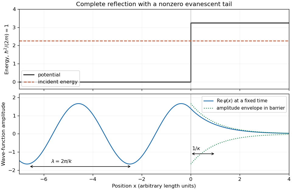
The wave-function amplitude decays as $e^{-\kappa x}$, so its e-folding penetration depth isThe probability density decays as $e^{-2\kappa x}$ and has the smaller e-folding depth $1/(2\kappa )$. Specifying which quantity decays avoids a factor-of-two ambiguity in the term penetration depth.

A stationary evanescent wave does not assign a classical trajectory or a real local speed inside the forbidden region. The dwell time in a semi-infinite potential step measures probability stored in $x>0$ divided by incident probability current. For incident amplitude one,This gives a time in terms of $m,E,V_0$ through the definitions of $k,\kappa$. A simpler dimensional estimate is the penetration length divided by the incident speed, $\Delta x/v_{\mathrm{in}}=m/(\hslash k\kappa )=\hslash /[2\sqrt{E(V_0-E)}]$. The dwell time equals $(2E/V_0)$ times that estimate. Different operational timing definitions need not agree; treating the imaginary under-barrier momentum as a real particle velocity would not justify a unique traversal time.

Using $m\simeq 4m_p$ and $T=15\mathrm{meV}$, the nonrelativistic de Broglie wavelength and speed areFor the square interferometer, the enclosed area projected into a vertical plane is $a^2\sin \theta$. The gravitational phase shift in matter-wave interferometry is $\Delta \phi =mg{a}^2\sin \theta /(\hslash v)$ to leading order in the small gravitational energy change. Thus rotation from horizontal to vertical changes the fringe count byOne way to see the phase is that the horizontal arms differ in gravitational potential energy by $mga\sin \theta$ for a flight time $a/v$. Which-path detection entangles the atom with distinguishable detector states. If those states are orthogonal and the path record is ignored, their coherence is lost and the interference fringes disappear. This is a loss of interference visibility, not a change in the atom's de Broglie wavelength.

For the macroscopic mass,The ideal fixed-momentum expression tends to infinity as $v\to 0$. An everyday localized object is not a perfectly coherent momentum eigenstate, however: its thermal and environmental momentum uncertainty remains nonzero, and decoherence rapidly suppresses spatially separated coherent alternatives. Merely setting the mean velocity to zero does not prepare an object with a macroscopic coherence length.

For a uniformly illuminated single slit of width $w$, the far-field amplitude is proportional to $\sin u/u$, with $u=\pi w\sin \vartheta /\lambda$. Its first zeros occur at $\sin \vartheta =\pm \lambda /w$. If the quoted peak width is the full width between those zeros, the small-angle geometry givesThe Fraunhofer diffraction approximation is appropriate since $w^2/(\lambda L)\ll 1$. If the supplied width instead meant a half-width or full width at half maximum, its numerical conversion factor would differ; the displayed answer states the first-zero convention explicitly.

The normalized linear polarization state is $|\theta ⟩=\cos \theta |H⟩+\sin \theta |V⟩$. A transmitted-photon count implements the projector $|\theta ⟩⟨\theta |$. The Born rule givesthe single-photon form of Malus's law, assuming ideal polarizers and detection.

For the product state $|H{⟩}_A|H{⟩}_B$, the two projection amplitudes multiply. ThereforeThe independent factors arise from this product input; they cannot be assumed for a general correlated pair state.

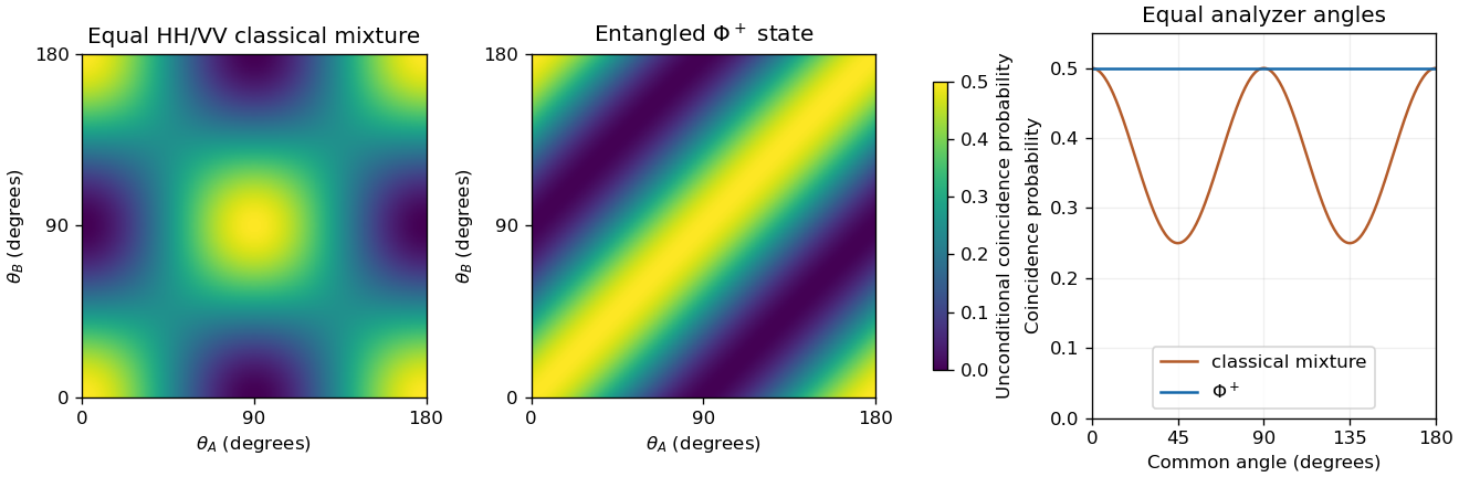
The classical mixture has density matrix $\rho =\frac{1}{2}|HH⟩⟨HH|+\frac{1}{2}|VV⟩⟨VV|$. Average the probabilities of its two alternatives:Alice's single-detector transmission probability is $1/2$ at every angle. Dividing by it givesAt $45^{\circ }$, Alice's click does not distinguish the two classical alternatives. At zero, it selects the horizontally polarized alternative.

The normalized Bell statehas equal outcomes for any common real linear-polarization basis. In the stated rotated basis it is $(|{\theta }^{(+)}{\theta }^{(+)}⟩+|{\theta }^{(-)}{\theta }^{(-)}⟩)/\sqrt{2}$: the cross terms cancel when the inverse rotation is substituted.

Thus the coincidence probability for the transmitted ports is $p(A,B)=\frac{1}{2}{\cos }^2({\theta }_A-{\theta }_B)$. At equal angles it is $1/2$ per emitted pair, while Bob transmits with probability one conditional on Alice's transmission. Both photons are blocked for the other half of ideal pairs. The phrase always in coincidence must therefore mean matching outcomes or conditional transmission, rather than unit unconditional transmission through both polarizers.

The classical mixture has no coherence between $HH$ and $VV$; it gives equal-angle coincidence probability $1/4$ at $45^{\circ }$, rather than $1/2$. The coherent quantum superposition maintains correlation in this rotated basis. Bob's unconditional transmission remains $1/2$, so the conditional correlation does not permit signalling by Alice's polarizer choice.

Hamilton's principle makes the action $S[q]={\int }_{t_1}^{t_2}L(q,\dot{q},t)dt$ stationary under variations vanishing at the endpoints. It need not be a strict minimum. Varying the action and integrating the velocity variation by parts givesThe endpoint term vanishes. Since the interior variations are arbitrary, the fundamental lemma of the calculus of variations yields

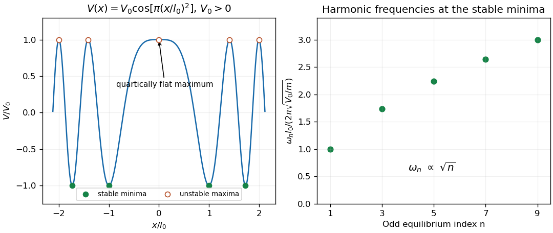
Write $u=\pi x^2/l_0^2$ and assume $V_0>0$. The derivative of the potential is $V^{\prime }(x)=-2\pi V_{0}x\sin u/l_0^2$. Its equilibrium positions are zero and $x=\pm l_0\sqrt{n}$ for positive integers $n$. At a nonzero equilibrium,Thus the stable equilibria and their small-oscillation normal mode frequencies areEven positive $n$ give unstable maxima. At zero the quadratic term vanishes but $V(x)=V_0-V_0{\pi }^2{x}^4/(2l_0^4)+\cdots$, so the equilibrium is still unstable; a zero linearized frequency does not prove stability. If the unspecified sign of $V_0$ were chosen negative, even-$n$ positions would be stable instead, together with a degenerate quartic minimum at zero whose frequency tends to zero with oscillation amplitude.

For an infinitesimal continuous symmetry $\delta q_i=\epsilon {\xi }_i(q,t)$, allow the Lagrangian to change by a total derivative, $\delta L=\epsilon dF/dt$. Direct variation givesOn a solution of the Euler-Lagrange equations, the first term vanishes. This proves Noether's theorem in the fixed-time form:Spatial translations yield total momentum, and rotations yield angular momentum. Time translations yield energy when the Lagrangian has no explicit time dependence; this follows either from the extended time-transformation form of the theorem or by differentiating $H={\sum }_i{p}_i{\dot{q}}_i-L$ to obtain $\dot{H}=-\partial L/\partial t$.