Past exam of the short options paper shared by Prelims and Parts A and B of the physics course of the University of Oxford / 2015 / S25 / 2

Use a positive stabilizing feedback coefficient: the net flux is $N=F_{\mathrm{ext}}-\lambda \Delta T$. The Planck feedback increases outgoing thermal radiation as temperature rises and therefore contributes positively to $\lambda$. Water-vapor feedback raises infrared opacity as a warmer atmosphere holds more water, tending to reduce $\lambda$; ice-albedo feedback also tends to reduce it as bright ice is lost. These signs depend on the explicitly stated convention.

For doubled carbon dioxide forcing $F_{2\times }>0$, equilibrium givesA symmetric positive interval $[{\lambda }_0-{\sigma }_{\lambda },{\lambda }_0+{\sigma }_{\lambda }]$ maps toThe upward excursion is larger than the downward one because inversion is nonlinear. If the interval reaches zero, it supplies no finite upper bound on equilibrium warming within this linear stable model.

Take the logarithmic forcing law with its normalization fixed by the given doubling value. Let $x$ be the positive magnitude of cooling and $f$ the positive magnitude of the earlier negative forcing:At $C=212\mathrm{ppm}$, $f_0=1.5051\mathrm{W}{\mathrm{m}}^{-2}$. Equilibrium then yieldsThe concentration endpoints $185$ and $244\mathrm{ppm}$ imply forcing magnitudes $2.242$ and $0.7445\mathrm{W}{\mathrm{m}}^{-2}$, approximately $f_0\pm 0.75$. Define normalized variables $u=f/f_0$ and $v=x/x_0$. Independent approximately Gaussian uncertainties give the one-standard-deviation covariance ellipseIts centre is $(1,1)$ and its principal directions are the two coordinate axes. Warming is $2.492(v/u)\mathrm{K}$, so rays from the origin have constant inferred warming. The bounding rays tangent to this ellipse have slopes $m$ satisfying $(1-m{)}^2=\frac{1}{4}(1+m^2)$, orThis gives the useful asymmetric one-parameter profile estimateThe concentration data supply only marginal intervals, not a full likelihood. This result explicitly approximates their logarithmic forcing uncertainty as Gaussian. Linear error propagation would instead give fractional uncertainty $\sqrt{0.5^2+0.5^2}=0.707$, or roughly $2.49\pm 1.76\mathrm{K}$, and misses the large reciprocal asymmetry. A unit-radius two-dimensional covariance ellipse itself contains about $39\%$ of a bivariate Gaussian, not $68\%$; the quoted interval uses the one-parameter $\Delta {\chi }^2=1$ profile/ratio construction, rather than claiming that ellipse is a $68\%$ joint region.

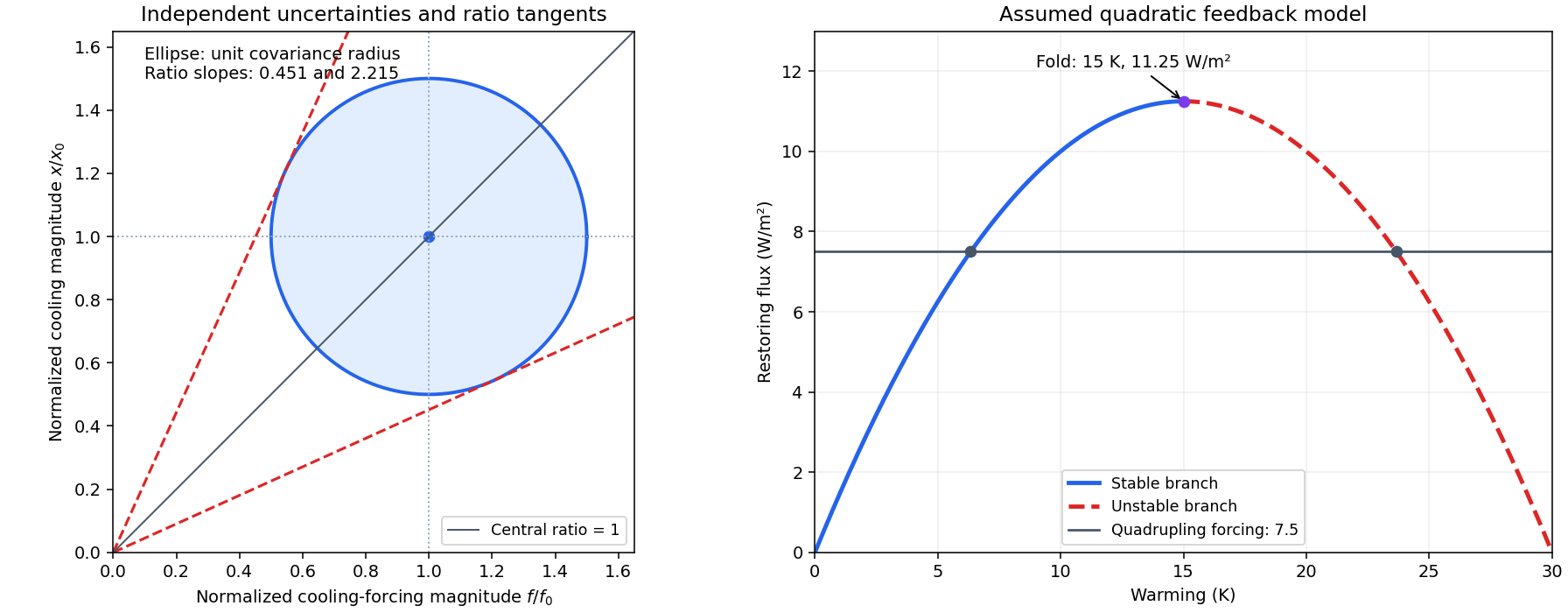
The quadratic coefficient must have units $\mathrm{W}{\mathrm{m}}^{-2}{\mathrm{K}}^{-2}$; the printed ${\mathrm{K}}^{-1}$ makes its term dimensionally incompatible with a radiative flux. Interpret its numerical value as ${\lambda }_2=0.05\mathrm{W}{\mathrm{m}}^{-2}{\mathrm{K}}^{-2}$, with ${\lambda }_1=1.5\mathrm{W}{\mathrm{m}}^{-2}{\mathrm{K}}^{-1}$. The total imbalance isA quadrupling gives $F_{\mathrm{ext}}=2(3.75)=7.5\mathrm{W}{\mathrm{m}}^{-2}$. The two equilibrium roots areFor positive heat capacity, stability requires $\partial N/\partial T=-{\lambda }_1+2{\lambda }_2\Delta T<0$. Thus only the lower root is stable. A saddle-node bifurcation occurs atThe logarithmic forcing relation gives $C_{\mathrm{crit}}=2802^{11.25/3.75}=2240\mathrm{ppm}$. Strict linear stability holds below this concentration on the lower branch; the equality is marginal and is the supremum, not another strictly stable equilibrium. Sustained forcing above it causes warming without a balancing equilibrium in this quadratic model. At such large changes its local feedback expansion can fail, and other physics can intervene; it does not prove unlimited real-planet warming or locate a measured Earth runaway threshold.