Short options paper shared by Prelims and Parts A and B of the physics course of the University of Oxford

The cover combines the preliminary examination and Parts A and B; candidates select the short options for which they have entered.

Source paper: www.whatdotheyknow.com/request/oxford_physics_past_papers_2/response/2340696/attach/6/Physics%20Papers%202017.pdf?cookie_passthrough=1

A branch point is a point around which analytic continuation changes the value of a multivalued function. For $z^{1/2}=r^{1/2}{e}^{i\theta /2}$, one circuit around zero changes the sign. A branch cut removes paths producing this ambiguity; for example $-\pi <\arg z<\pi$ gives a single holomorphic square root off the nonpositive real axis. The position of a cut is a convention, while the branch point is intrinsic.

Set $q(z)=(z-1)/(z+1)$. For $z$ outside the closed segment joining $-1$ to $1$, $q(z)$ avoids the nonpositive real axis. Therefore the principal square root of $q$ defines a holomorphic function there, with the normalization $f(\infty )=1$. The endpoints are branch points. Expanding at infinity,For a positively oriented contour surrounding the cut, its integral equals the integral on a sufficiently large positively oriented circle, since the intervening annulus is holomorphic. ThusOn the upper and lower banks, $f_{+}(x)=+i\sqrt{(1-x)/(1+x)}$ and $f_{-}(x)=-i\sqrt{(1-x)/(1+x)}$. The upper bank is traversed from $1$ to $-1$, and the lower bank from $-1$ to $1$. Their sum is $-2i$ times the required real integral. Small endpoint arcs vanish because their singularities have exponent less than one. ConsequentlyFor $\alpha =1/n$, use $f_{\alpha }=q^{\alpha }$ with the same normalization. Its expansion is $1-2\alpha /z+O(z^{-2})$, and its bank values are $e^{\pm i\pi \alpha }[(1-x)/(1+x){]}^{\alpha }$. Equating the contour integral $-4\pi i\alpha$ with $-2i\sin (\pi \alpha )$ times the real integral givesThe condition $n\ge 2$ ensures endpoint integrability. Choosing the other square-root branch reverses $I_{\Gamma }$, but also reverses both bank values, leaving the real integral unchanged.

Integrate $e^{iz}/z$ around an upper semicircle, indenting the origin by a small upper semicircle traversed clockwise. The integrand is holomorphic inside the indented contour. The large arc vanishes by Jordan's lemma, and the small arc contributes $-i\pi$, soTaking imaginary and real parts yieldsThe first integrand has a removable singularity at zero and its tails converge conditionally by Dirichlet test for improper integrals. The second integral needs a principal value at zero; its zero also follows from oddness with symmetric exclusion. One must not assign an ordinary convergent integral to its singularity.

Put $z=e^{i\theta }$, so $\sin \theta =(z-z^{-1})/(2i)$ and $d\theta =dz/(iz)$. The integral becomesThe poles are $-2i/3$ and $-3i/2$; only the first is inside the unit circle. The derivative of the denominator there is $12(-2i/3)+13i=5i$. The residue theorem therefore givesThere are no poles on the contour because the real denominator is at least one.

At a regular point, $f(z_0+\zeta )-f(z_0)=f^{\prime }(z_0)\zeta +O({\zeta }^2)$. Multiplication by a nonzero complex number rotates every tangent by the same angle and multiplies every length by the same positive factor. Oriented angles are preserved. If the first derivative vanishes but the second does not, the leading term is $f^{\prime \prime }(z_0){\zeta }^2/2$: tangent arguments are doubled, so angles are doubled, modulo the identification of rays. This is a local statement; holomorphy alone does not imply global injectivity.

Write $z=x+iy$. ThenFor $-1<x<1$ and $y>0$, the imaginary part is positive. The bottom edge maps monotonically to $[-1,1]$; the left and right vertical edges map to $(-\infty ,-1]$ and $[1,\infty )$ respectively. The inverse below establishes that every point of the open upper half-plane occurs exactly once. At fixed $y=a$, putting $u=\mathrm{Re}w$, $v=\mathrm{Im}w$, one obtainsThis is the upper half of an ellipse, traversed from its left endpoint to its right endpoint.

Choose the branch $s(w)=\sqrt{1-w^2}$ analytic in the upper half-plane and positive on the boundary interval $(-1,1)$. Then the inverse branch into the strip isThe logarithm is chosen continuously so that $-1<\mathrm{Re}z<1$ and $\mathrm{Im}z>0$; for instance $w=iv$, $v>0$, gives $z=(2i/\pi )\mathrm{arsinh}v$. Differentiation gives $dz/dw=2/(\pi \sqrt{1-w^2})$. The only zeros of the original derivative in the closed strip are $z=\pm 1$, with images $w=\pm 1$. The inverse has square-root branch points there, and cannot extend holomorphically across them. At either corner the original map doubles the right angle to a straight angle; a holomorphic inverse with nonzero derivative could not halve it. The open strip interior has no such failure.

The distance modulus at $100\mathrm{pc}$ is five magnitudes. Thus the two approximate main-sequence endpoints read from the original figure, $m_V\simeq 0,20$, correspond to $M_V\simeq -5,15$. With the given solar reference,Use the figure's approximate endpoint effective temperatures $25,000$ K and $2500$ K. If $V$-band luminosity is used as a rough bolometric proxy, the Stefan–Boltzmann law givesTaking $T_{\odot }\simeq 5800$ K givesThese are schematic estimates, not precision radii. The diagram supplies $V$ magnitudes rather than bolometric luminosities, and hot and cool endpoints need different bolometric corrections. The exact range cannot be recovered without those corrections; the quoted values state the intended approximation explicitly.

Integrating $dP/dr=-G{M}_r\rho /r^2$ in order of magnitude, with $\rho \sim M_{\ast }/R_{\ast }^3$, givesThe ideal gas law independently gives $P_c\sim M_{\ast }{k}_B{T}_c/(\mu m_H{R}_{\ast }^3)$. Equating the two estimates yieldsFor similar composition and an approximately fixed hydrogen-burning central temperature, $R_{\ast }\propto M_{\ast }$. Calibrating this rough relation on the Sun and using part a gives a nominal mass range of about $0.05$ to $5M_{\odot }$.

The endpoint luminosity ratio is $10^8$, whereas the inferred mass ratio is about $10^2$, giving $L\propto M^4$ across that range. The exponent is therefore consistent at this schematic level. The solar normalization and individual endpoint masses are much less reliable: using the luminosity relation itself gives approximately $0.1$ to $10M_{\odot }$. Central temperatures are not truly constant, low-mass stellar structure differs, and the uncorrected $V$ luminosities in the diagram are not bolometric. These limitations prevent treating the rough radius-based masses as a contradictory precision measurement.

If radiation dominates the central pressure, equate $P_c\sim G{M}_{\ast }^2/R_{\ast }^4$ to $a{T}_c^4/3$. This givesAt roughly fixed burning temperature, the corresponding mass-radius scaling is $R_{\ast }\propto M_{\ast }^{1/2}$, rather than the gas-pressure estimate $R_{\ast }\propto M_{\ast }$. Radiation pressure alone does not determine a unique radius at a specified mass: a thermal or nuclear-burning condition is still needed to specify $T_c$. The relation is a homology estimate, not a universal exact law for all massive stars.

The numbered features in the original colour-magnitude diagram have the following interpretation.

Continuous star formation explains the coexistence of newly formed massive main-sequence stars with evolved low-mass remnants; interpreting a single sharp turnoff as the age of a coeval cluster would be inappropriate here.

At this small redshift, $D\simeq cz/H_0\simeq 20.0$ Mpc. The outer angular radius gives $R_{\mathrm{out}}\simeq D\theta \simeq 21.3$ kpc. Approximating the dynamical mass by a spherical equivalent,The supplied Tully-Fisher relation gives $M_V\simeq -22.49$, and hence $L_V\simeq 9.9\times 10^{10}{L}_{V,\odot }$. Treating the population as solar-like gives the estimate ${{\rm Y}}_V\simeq 1M_{\odot }/L_{V,\odot }$, soThe dynamical estimate exceeds that by about a factor of five; a massive extended dark-matter component is the natural interpretation. Solar-like spectra do not exactly fix the population mass-to-light ratio, and a disk is not spherical, but order-unity corrections do not remove this large outer mass excess under the stated estimate.

The effective radius is one tenth of the optical outer radius: $R_e\simeq 2.13$ kpc. A flat rotation speed then gives $M_{\mathrm{dyn}}(<R_e)\simeq 4.9\times 10^{10}{M}_{\odot }$. Half the luminosity, with the same mass-to-light ratio, implies $M_{\mathrm{luminous}}(<R_e)\simeq 4.9\times 10^{10}{M}_{\odot }$.The concentration of light into a small fraction of the optical radius suggests a high-surface-brightness, centrally concentrated disk galaxy, plausibly an early-type spiral or lenticular with a substantial bulge. The kinematic and photometric data do not uniquely distinguish those morphologies. Disk geometry, an unknown inclination correction, or a varying stellar mass-to-light ratio would alter the exact numerical inner comparison.

Using the same luminosity estimate, the distance modulus is $12.5-(-22.49)=34.99$, implying $D\simeq 99.4$ Mpc. Pure Hubble expansion at that distance predicts about $7450\mathrm{km}{\mathrm{s}}^{-1}$. The measured velocity therefore impliesIts line-of-sight peculiar velocity is toward us, of the order expected for orbital motions in a rich galaxy cluster. A galaxy falling toward a cluster centre from its far side could have this sign. Its actual front/back location or three-dimensional orbit is not determined without the cluster's mean velocity, distance and projected position. Tully-Fisher scatter and the assumption of identical luminosities also limit that inference.

Let $I$ denote a characteristic surface brightness and ${\rm Y}=M/L$ the relevant dynamical mass-to-light ratio. With comparable profiles, $L\propto I{R}^2$ and $M\propto V^{2}R/G$. Eliminating $R$ givesIf both $I$ and ${\rm Y}$ are independent of speed, converting luminosity to magnitude gives $M_V=\text{constant}-10{\log }_{10}V$. The empirical coefficient $-8$ instead means $L\propto V^{3.2}$, and thereforeFor constant surface brightness this requires ${\rm Y}\propto V^{0.4}$; for constant mass-to-light ratio it requires $I\propto V^{0.8}$. A mixture of these changes, including varying stellar populations or dark-matter fractions, can give the same observed slope. The simple derivation assumes comparable characteristic radii and structural coefficients.

The curvature constant specifies the intrinsic spatial curvature of homogeneous constant-time slices. Positive curvature has spherical geometry, zero curvature Euclidean geometry, and negative curvature hyperbolic geometry. A conventional coordinate normalization uses $k=+1,0,-1$, with the scale factor carrying the curvature radius; rescaling that factor changes the numerical magnitude assigned to a dimensional curvature coefficient.

The sign alone does not determine the future expansion once a cosmological constant is admitted. Nor does negative or zero local curvature by itself determine the global topology: quotient spaces can share the same local curvature.

For conserved nonrelativistic matter, ${\rho }_M={\rho }_{M0}{a}^{-3}$, where $a=R/R_0$ and $a_0=1$. Substitution into the Friedmann equation giveswithThe source writes the dimensionless normalized factor as $R$ in its final expression; this is equivalent to setting $R_0=1$ consistently in the curvature coefficient. Evaluating today gives ${\Omega }_M+{\Omega }_k+{\Omega }_{\Lambda }=1$. Here the printed $\Lambda$ already has dimensions of inverse time squared. If the cosmological constant is instead defined geometrically with inverse-length-squared units, replace this $\Lambda$ by ${\Lambda }_{\mathrm{geom}}{c}^2$.

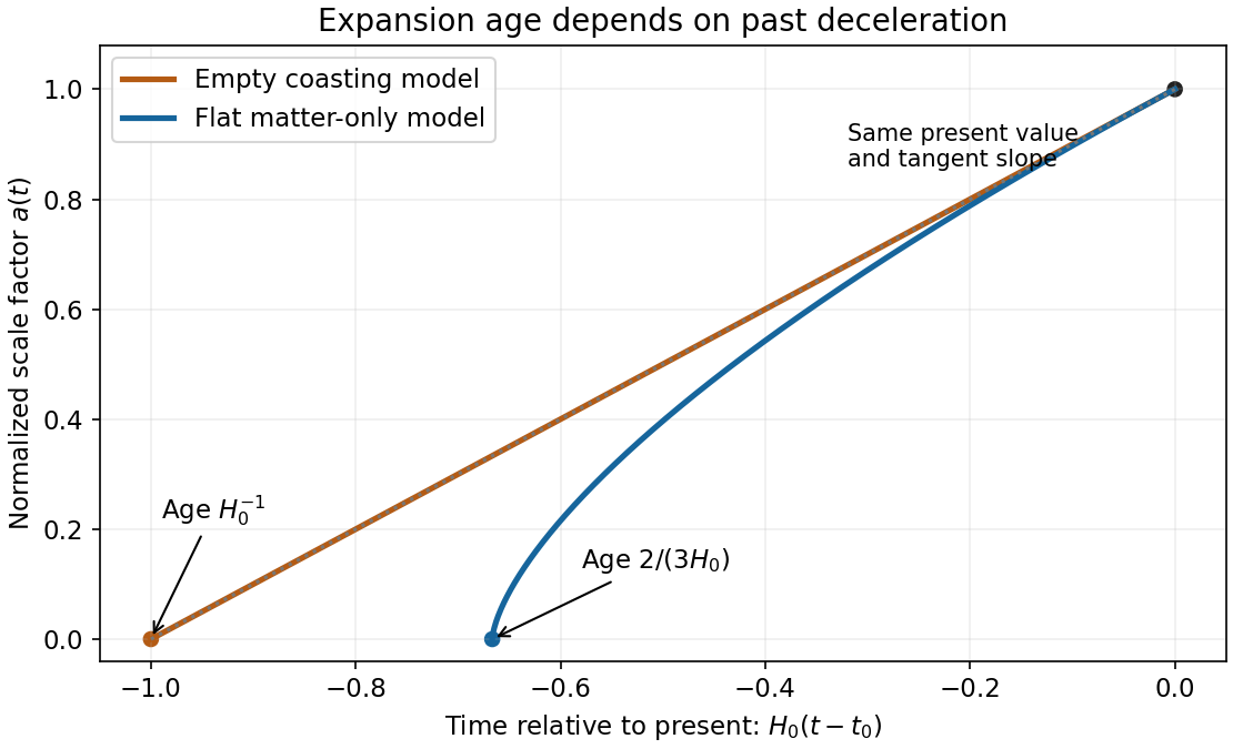
With zero curvature and no cosmological constant, the present normalization requires ${\Omega }_M=1$. Thus $\dot{a}=H_0{a}^{-1/2}$, and choosing the big bang as $t=0$ givesFor an empty expanding model, ${\Omega }_k=1$ and the curvature must be negative. The equation becomes $\dot{a}=H_0$, givingThe latter is the Milne slicing of flat spacetime; its zero-scale-factor origin is not a matter-density curvature singularity. In the matter model, gravity decelerates expansion, so the earlier slope was greater than the present slope and the same present size was reached in less time. With the stipulated $H_0$, the two model ages are approximately $8.69$ and $13.0$ Gyr.

Adiabatic photon redshifting gives $T\propto a^{-1}$. Using the stipulated temperatures,In the flat dust approximation of part c, $t=t_0{a}^{3/2}$, so $t_{\mathrm{rec}}\simeq (2/3H_0)1000^{-3/2}\simeq 2.75\times 10^5$ years. This approximation omits the significant radiation contribution near the actual recombination epoch.

The elementary travel-distance estimate is $c{t}_{\mathrm{rec}}\simeq 8.4\times 10^4$ pc, whose corresponding comoving scale today is about $84$ Mpc. In an expanding universe, however, that is not the exact proper particle-horizon radius. Integrating the null geodesic givesfor dust. Thus the proper horizon at this epoch is about $0.25$ Mpc and its present comoving size about $250$ Mpc. The factor three accounts for expansion during light propagation. These scales describe the limited causal domain in the simple decelerating model. The near-uniform CMB temperature across much more widely separated last-scattering regions motivates the horizon problem; the question's rough $ct$ estimate and the exact dust horizon should not be conflated.

The de Broglie hypothesis associates a wave phase with a material particle. Its momentum and energy setThis is not a literal extended classical lump of matter oscillating at every point. A wavefunction gives amplitudes for measurements, and a localized particle is represented by a superposition of momentum waves. Electron diffraction, for example, exhibits interference at angles set by the same wavelength relation.

Using the given one-component equipartition estimate, $p^2=M{k}_{B}T$. Substituting into the de Broglie relation givesComparison with a confinement length or interparticle spacing $d$ gives the criterion $T\lesssim h^2/(M{k}_B{d}^2)$. Numerical factors depend on the convention: the statistical thermal de Broglie wavelength is usually $h/\sqrt{2\pi M{k}_{B}T}$, while a three-component root-mean-square momentum introduces a factor $\sqrt{3}$. The question's specified one-component convention is used consistently here. Once degeneracy becomes important, classical equipartition itself ceases to describe the electrons accurately.

Set $\lambda \simeq d$ with the convention of part b. ThenThus ordinary solid-state temperatures are far below this rough overlap scale. The electrons need quantum statistics and quantum states throughout that regime. The number is an order-of-magnitude wavelength criterion, not an exact Fermi temperature: electron density, electronic band structure, effective mass and the numerical convention all matter.

At the same temperature, momenta increase as the square root of mass, so wavelengths decrease as its inverse square root. For a nucleus of mass $M_N\simeq A{m}_p$,At the electron overlap threshold, ${\lambda }_e=d$, the nuclear wavelength is about $7.0\mathrm{pm}/\sqrt{A}$, far below the $0.3$ nm spacing. Nuclear exchange effects are consequently much less important than electron exchange effects. This statement about nuclear overlap does not mean lattice vibrations are always classical.

At room temperature, electrons require quantum mechanics, including their occupied orbitals or bands and Fermi statistics. Heavy nuclei can often be treated as distinguishable particles near classical equilibrium lattice sites, because their exchange wavelengths are short. Their coupled displacements form phonons, however, and the occupation of a vibrational mode is classical only if $k_{B}T\gg \hslash \omega$ for that mode. Even at room temperature some high-frequency modes remain quantum mechanical.

At $1$ K, quantum lattice vibrations, zero-point motion and the scarcity of thermally excited phonons are essential. Many heavy nuclei still do not have overlapping exchange wavefunctions; quantum vibration and quantum exchange are distinct criteria. For the same spacing, the nuclear overlap threshold from the rough estimate is $T_N\simeq 211/A$ K, illustrating why the nuclear mass cannot be omitted from a blanket low-temperature claim.

Choose the overall phase so that $A$ is positive. Normalization requiresThereforeAn arbitrary constant phase multiplying this answer has no effect on any expectation value.

The probability density is even, so its first moment vanishes. Its second moment follows by integrating the polynomial:Using the normalization from part a givesThe variance in position is consequently $a^2/7$.

The wavefunction is real and vanishes continuously at both endpoints. HenceThe momentum second moment is most safely evaluated from its quadratic form:ThusThe derivative jumps where the wavefunction joins zero. On the whole real line the strong second-derivative operator therefore produces endpoint delta distributions, so the state is not in the usual operator domain of $p^2$. The finite momentum second moment, equivalently the kinetic-energy quadratic form or the integral of $p^2$ against the momentum probability density, remains well defined and gives the value above.

Both first moments vanish, so the standard deviations follow directly from the second moments:The Heisenberg uncertainty relation is satisfied and is not saturated. A Gaussian wave packet can saturate the position-momentum bound; this compactly supported polynomial is not Gaussian.

For a single slit of width $d$, the far-field amplitude is proportional to $\mathrm{sinc}(\pi d\sin \theta /\lambda )$. The first zeros satisfy $d\sin \theta =\pm \lambda$. At small angles the angular width between those zeros is $2\lambda /d$, or $2L\lambda /d$ on a screen a distance $L$ away.The result assumes the wavelength, propagation distance and far-field conditions stay fixed. If the slit becomes comparable to the wavelength, the exact sine relation replaces the small-angle scaling.

Quantum tunnelling is transmission through a region where the particle's energy is below the classical potential energy. The stationary wavefunction decays within that region but need not vanish at its far boundary, so matching can leave a nonzero transmitted probability current.

This does not require a particle to borrow energy temporarily. Energy is conserved for a time-independent barrier; the classically forbidden region is described by an evanescent wave, with the same stationary energy as the incident and transmitted waves.

Inside a rectangular barrier with $E<V$, the stationary Schrödinger equation givesIts independent solutions are $e^{\pm \alpha x}$ withFor an opaque barrier the amplitude is suppressed by approximately $e^{-\alpha L}$ and the probability by $e^{-2\alpha L}$. Matching contributes a prefactor, so this exponential approximation is not an exact transmission coefficient for a transparent or very thin barrier. For two moving particles the relative-coordinate mass is their reduced mass.

At a separation of $1$ fm, the proton Coulomb energy is approximately $V=e^2/(4\pi {\epsilon }_{0}r)\simeq 1.44$ MeV, whereas $k_{B}T\simeq 0.862$ keV at the stated solar-core temperature. As a deliberately crude rectangular-barrier estimate, take a width of $1$ fm and use the two-proton reduced mass $\mu =m_p/2$. ThensoTreating one proton as fixed and using $m_p$ instead gives about $0.59$. Both estimates only say that this arbitrarily shortened barrier would be fairly transparent; the opaque-barrier exponential is itself uncontrolled for such a small exponent.

There is an important conditioning issue. If the protons have already reached a separation of one femtometre, most of the long-range Coulomb suppression has already been overcome. The rectangular estimate cannot represent the probability for thermal protons starting far apart. Their classical turning separation at this energy is about $1.7\times 10^3$ fm, not one femtometre.

Two major suppressions are missing from the one-femtometre rectangular estimate. First, the Coulomb barrier extends far beyond nuclear distances and is not rectangular. A semiclassical integral through it produces the Gamow factor $\exp (-2\pi \eta )$, with $\eta ={\alpha }_{\mathrm{fs}}\sqrt{\mu c^2/(2E)}$; at the illustrative thermal energy it is already of order $10^{-11}$. A thermal average additionally weights the high-energy tail and is not the same as evaluating a single thermal energy.

Second, two protons cannot simply form a stable bound diproton. The proton–proton chain starts with a weak-interaction conversion producing a deuteron, a Positron and a neutrino. The weak transition probability supplies a further very large suppression. Thus the quoted tiny fusion probability is not a pure one-dimensional barrier transmission probability with universal energy-independent meaning.

The Sun contains of order $10^{57}$ nucleons in a hot dense core and offers enormously many encounters over astronomical times. A very small reaction probability per encounter can therefore supply its luminosity while consuming only a small fraction of the fuel per unit time. The small weak reaction rate is also crucial for the long stellar lifetime; a larger core temperature increases burning and triggers expansion and cooling.

The Shockley-Queisser calculation treats a single-junction solar cell with a single band gap, in steady state, with one collected electron-hole pair per absorbed above-gap photon, an ideal absorption edge, thermalized carriers and radiative recombination as the limiting recombination process. The source spectrum, cell temperature, angular acceptance and optical concentration must be specified. Below-gap photons are transmitted; energy above the gap is lost during carrier thermalization; the cell must emit photons by detailed balance, producing a recombination current and an entropy-related voltage loss. Delivering power at finite current also puts the operating voltage below the open-circuit voltage. Nonradiative recombination, resistance and imperfect collection worsen a real cell but are not required for the ideal limit.

Three ways to change those assumptions are tandem solar cells, which divide the spectrum among gaps and reduce both transmission and thermalization losses; hot-carrier solar cells, which aims to collect excess carrier energy before thermalization; and carrier multiplication or spectral conversion, which aims to use a high-energy photon for more than one excitation or combine otherwise unusable sub-gap photons. These concepts have additional practical losses and do not automatically outperform an optimized conventional device. The usual unconcentrated single-junction optimum is approximately one third under a terrestrial solar spectrum, rather than a universal efficiency independent of illumination.

For the geometrical estimate, take the stated horizontal equinox irradiance to set a constant direct-normal reference. The equinox solar-noon elevation is ${\alpha }_e=90^{\circ }-51.75^{\circ }=38.25^{\circ }$, so this reference is $I_n=1/\sin {\alpha }_e\simeq 1.62\mathrm{kW}{\mathrm{m}}^{-2}$. A south-facing panel with tilt $\beta =41.1^{\circ }$ has noon incidence factor $\cos (51.75^{\circ }-\delta -41.1^{\circ })$, where $\delta =\pm 23.44^{\circ }$. Relative to the $1\mathrm{kW}{\mathrm{m}}^{-2}$ plane-of-array rating,These are the results of that idealized geometrical normalization, not credible seasonal production forecasts. Its inferred direct-normal irradiance already exceeds the approximately $1.36\mathrm{kW}{\mathrm{m}}^{-2}$ solar irradiance outside the atmosphere, so the supplied horizontal benchmark cannot describe a purely direct noon beam literally. Real direct and diffuse fractions, atmospheric attenuation at low winter elevation, cell temperature and inverter clipping are unspecified. An alternative assumption of $1\mathrm{kW}{\mathrm{m}}^{-2}$ direct-normal irradiance gives approximately $4.88$ and $4.14$ kW. A physically unique maximum cannot be inferred without an irradiance model.

The stated annual output corresponds to $4100/5=820$ full-rated hours, an average power of $0.468$ kW and a capacity factor of $9.4\%$. Night, cloud, seasonal day length and other losses explain the large difference from an instantaneous sunlit estimate.

For a national scale estimate, take UK area $2.44\times 10^{11}{\mathrm{m}}^2$, population $6.6\times 10^7$, and annual mean solar input $100\mathrm{W}{\mathrm{m}}^{-2}$. Covering five percent with twenty-percent-efficient modules givesThis is comparable with an order-$100$ kWh daily per-person primary-energy budget, and much larger than electricity use alone, of order $10$-$15$ kWh per person per day. It is a gross area-and-flux estimate: access land, shading, seasonal storage, curtailment and conversion between primary energy and electrical end use all affect its interpretation.

A pumped-storage plant moves water uphill using electrical power, then returns it through a turbine and generator when electricity is needed. The upper and lower reservoirs set the usable volume and head; pumps, penstocks, valves and reversible pump-turbines set the power and flow. The plant stores energy rather than generating net energy over a cycle.

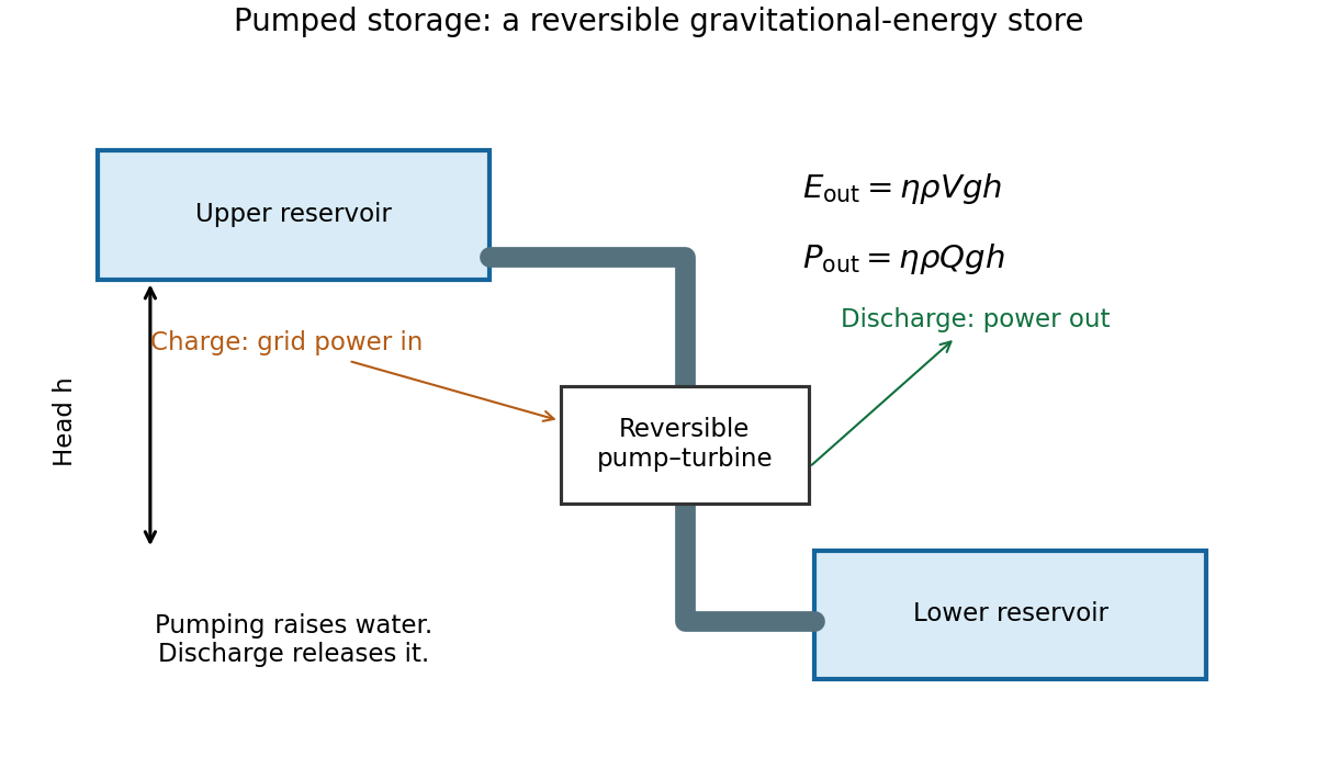
For constant head, the gravitational energy is $E_g=\rho Vgh$. With the stated generation efficiency,At $3$ GW, $P=\eta \rho gQh$ givesHead variation, dead volume and hydraulic losses beyond the stipulated efficiency have been neglected.

To deliver $9$ kWh with the same head and efficiency needs $V\simeq 9.3{\mathrm{m}}^3$ of water, roughly a $2.1$ m cube, together with a $400$ m elevation difference and a lower reservoir. At a $10$ m head it would need about $370{\mathrm{m}}^3$. This contrasts with the small fuel volume: the useful energy density of lifted water depends on its external head, not its chemical composition.

Pumped storage offers long service life, fast dispatch, substantial power, and separate choices of storage volume and turbine rating. Its drawbacks include geographic constraints, construction cost and time, ecological impacts, evaporation and water requirements, plus round-trip losses. The quoted generation efficiency alone is not the round-trip efficiency because pumping also consumes more than the stored potential energy.

The rock cylinder has mass ${\rho }_r\pi r^2(2r)$ and rises through $r$. Equating its useful energy to the reservoir result cancels the common efficiency and gravity:Its height is about $262$ m and its lift about $131$ m, ignoring buoyancy as instructed. Stored energy scales as $r^4$, excavated volume roughly as $r^3$, and lined area as $r^2$. If excavation dominates cost, cost per unit stored energy decreases approximately as $r^{-1}$. Seals, increasing pressure, geology, leakage, supporting structure and power equipment can change that scaling; a volume law is not a complete cost model.

Fission divides a heavy nucleus into more tightly bound fragments, releasing energy through the increase in binding energy per nucleon. A neutron-induced chain reaction can sustain heat production in a controlled reactor. Fusion combines light nuclei into more tightly bound products and needs sufficiently high temperature and confinement to obtain a useful reaction rate despite Coulomb repulsion. Both ultimately supply heat that must be converted to electricity, unless a different energy-conversion scheme is explicitly introduced.

A typical fission releases about $200$ MeV per event, corresponding to roughly $8\times 10^{13}$ J per kilogram of fully fissioned heavy fuel. The deuterium-tritium fusion energy of $17.6$ MeV per reaction corresponds to about $3.4\times 10^{14}$ J per kilogram of reacting mixture. These are nuclear reaction energies, not electricity per kilogram of mined or engineered fuel. Actual fuel use, thermal efficiency, parasitic power and incomplete burn change plant output.

Fission has substantial operating experience and can provide high-capacity-factor generation, but faces capital, waste, decommissioning, fuel-cycle and safety constraints. Fusion avoids a self-sustaining neutron chain reaction in the fuel, but its systems still face neutron damage, activated materials, tritium management and demanding heat extraction. Demonstrating a hot plasma or a favorable reaction-energy balance is not the same as demonstrating economical net electricity. The useful comparison distinguishes scientific feasibility, engineering availability and whole-system cost.

Distributed generation changes the shape of infrastructure rather than eliminating it. A $1$ GW power station is large, but supplying a national mean demand of tens of gigawatts from smaller intermittent generators still requires transmission, distribution, power conversion, forecasting, balancing and often storage or dispatchable reserve. Geographic diversity can reduce weather correlations only if power can move between regions.

For scale, delivering $30$ GW through a network is a continuous transfer of $30$ billion joules each second. Even a distributed average installation of $3$ kW per household needs ten million participating households to reach that power, before allowing for capacity factor. Solar roofs can reduce some local flows while export peaks or winter deficits increase others. District heat, offshore wind connections, interconnectors and fuel transport also have economies of scale.

Large centralized assets can introduce single-point failure, slow construction and financing risk; modular systems can be installed incrementally and offer local control. Conversely, network reinforcement and seasonal adequacy cannot be inferred from the size of an individual panel. A defensible conclusion is that an effective mix may combine small generators with large shared infrastructure. The categorical claim that large-scale infrastructure has become obsolete does not follow from the existence of distributed generation.

Compare average delivered electrical power per land area with consistent boundaries. Illustrative values are about $1000\mathrm{W}{\mathrm{m}}^{-2}$ for the compact plant site of nuclear generation, $5$-$15\mathrm{W}{\mathrm{m}}^{-2}$ for a UK ground-mounted photovoltaic site, $1$-$3\mathrm{W}{\mathrm{m}}^{-2}$ across a wind-farm lease area, around $0.5\mathrm{W}{\mathrm{m}}^{-2}$ for an energy crop after conversion, and perhaps $5\mathrm{W}{\mathrm{m}}^{-2}$ for a reservoir hydroelectric scheme. These are scale estimates, not universal technology constants.

At representative values $1000,10,2,0.5,5\mathrm{W}{\mathrm{m}}^{-2}$, one average gigawatt requires approximately $1,100,500,2000,200\mathrm{k}{\mathrm{m}}^2$ respectively. Biomass therefore has substantial land competition even when fuel can be stored. Solar development competes less with farming if placed on roofs or already developed land. Wind's large separation area is not entirely excluded from agriculture; its actual foundations and roads occupy a much smaller area. Reservoir impacts can be extensive and strongly site dependent.

A nuclear-site number excludes mining, cooling constraints, transport and exclusion areas; a wind lease number includes much land still usable for other purposes. Reporting them as identical measures of permanently occupied land would mislead. Deployment decisions need both the average energy yield and the consequences of the particular land boundary, ecology, food production and local acceptance.

A battery stores electrochemical free energy. Representative pack specific energy is of order $0.1$-$0.25$ kWh/kg, with electrical round-trip efficiency roughly $85$-$95\%$. It responds rapidly and can be modular, but energy capacity requires more active material, and ageing depends on time, temperature and cycling.

Pumped storage stores gravitational potential energy. At a $400$ m head with $89\%$ generation efficiency, useful energy is $\eta gh\simeq 0.97$ Wh/kg of water. Its low mass-specific energy is acceptable when inexpensive water and large reservoirs are available. Storage volume and generator rating can be chosen substantially independently, making multi-hour service practical, but suitable sites and civil works are major constraints.

Hydrogen stores chemical energy, with a lower heating value around $33$ kWh/kg of hydrogen before allowing for tank mass. Electrolysis, compression or other storage processing, and conversion back to electricity can reduce electrical round-trip efficiency to roughly $25$-$45\%$, depending on the route. Separate tanks or caverns can make long-duration energy capacity less expensive than adding electrochemical cells, but containment, infrastructure, leakage and conversion equipment matter.

The appropriate comparison includes power rating, energy duration, cycle count, system mass or area, and whether heat or electricity is the final useful product. A large fuel heating value does not imply a high electricity-storage efficiency.

An experience curve models unit cost as $C(Q)=C_0(Q/Q_0{)}^{-b}$, where $Q$ is cumulative production. A doubling reduces cost by a fraction $1-2^{-b}$. For an illustrative twenty-percent reduction per doubling, $b=-{\log }_2(0.8)\simeq 0.322$, so four doublings would reduce the fitted cost to $0.8^4\simeq 0.41$ of its initial value.

Photovoltaic modules are manufactured in large numbers with repeated designs, so manufacturing yield, scale, automation and material use can all produce observable learning. Wind turbines also benefit from repeated manufacture, but installation, foundations, access, grid connection and site quality form a larger project-specific share; moving into poorer or more difficult sites may offset improvements. Nuclear reactors have fewer repetitions, long project times, changing designs and regulation, and substantial site and financing costs. A cumulative-capacity curve can therefore hide rather than explain changes in nuclear project cost.

A experience curve is an empirical conditional relationship, not a physical law guaranteeing success. Input prices, policy, financing, saturation of a manufacturing improvement and the definition of system boundary all affect extrapolation. Declining cost may encourage deployment, which then increases the cumulative-production variable, so correlation alone does not establish a one-way causal effect. Forecasts should test multiple learning rates and distinguish module or turbine cost from the cost of a reliable delivered electricity system.

Take a fully backed-up peak demand of $60$ GW, an illustrative gas capacity capital cost of £$500$/kW, and an annual capital-recovery factor of $0.10$. The installed cost is £$30$ billion, so the annual capital charge is £$3$ billion. Spread over an illustrative annual electricity consumption of $300$ TWh,A doubled capital-cost assumption doubles this charge. This estimate counts backup capacity even if it runs rarely, which is why capital rather than fuel can dominate its fixed annual cost.

It is not the total cost of a renewable or gas system. Fuel, emissions, maintenance, staffing, gas supply during correlated cold weather, network capacity, startup constraints and reliability standards remain additional considerations. Backup requirements need not equal the sum of intermittent nameplate ratings; demand correlation, capacity credit, interconnection and storage matter. The arithmetic shows that a large reserve power rating can have a modest annualized capital charge per unit of total electricity, while leaving substantial practical and environmental constraints unresolved.

Use a conventional car consumption of $6$ litres per $100$ km and the supplied fuel-energy scale of $9$ kWh/litre. Driving $20,000$ km then consumes approximately $1200$ litres or $10,800$ kWh of fuel energy. If an energy-crop route delivers a net usable fuel power of $0.5\mathrm{W}{\mathrm{m}}^{-2}$ averaged over the year, its yield is $4.38\mathrm{kWh}{\mathrm{m}}^{-2}\mathrm{y}{\mathrm{r}}^{-1}$, requiring about $2500{\mathrm{m}}^2$ per car.

For an electric car consuming $0.18$ kWh/km, the annual electrical requirement is $3600$ kWh. With an annual incident solar energy of $1000\mathrm{kWh}{\mathrm{m}}^{-2}$ and module efficiency $20\%$, the module-area estimate isAllowing for spacing, charging and storage losses increases the solar land requirement, perhaps to several tens of square metres, while crop yield and processing losses change the biofuel estimate. Even with such corrections the difference can be many tens to over a hundredfold. The comparison includes the electric drivetrain's lower required input energy rather than incorrectly demanding equal fuel heating value from both routes. Agricultural land competition, biodiversity, fertilizer and indirect land-use change also matter for biofuels; solar infrastructure still needs material and seasonal-system assessment.

Only $A_z$ depends on position. Taking the curl,The field reverses across $x=0$. Its divergence is zero, as required for a magnetic field; the vanishing field on the midplane is important for the crossing and separatrix trajectories below.

With zero scalar potential, the nonrelativistic charged-particle Lagrangian in SI units is kinetic energy plus $q\mathbf{A}\cdot \dot{\mathbf{r}}$. ThusThe velocity-dependent magnetic term changes canonical momentum but does not contribute to the mechanical energy.

Define $a=q{B}_0/(2L)>0$. Differentiating the Lagrangian with respect to each generalized velocity givesThe coordinates $y$ and $z$ are cyclic, so $p_y$ and $p_z$ are conserved. The momentum $p_x$ is generally not conserved: its equation is ${\dot{p}}_x=-2ax\dot{z}$. In particular, conserved canonical $p_z$ is not the same as conserved mechanical $m\dot{z}$, which changes as the particle moves across the magnetic-field gradient.