Let . It is a nonnegative extended random variable, and implies . Otherwise its expectation would be infinite. Intersect this event with the countably many probability-one events on which the individual sample paths are continuous.
For every path in that intersection, . The Weierstrass M-test gives absolute and uniform convergence of on the entire stated time domain. A uniform limit of continuous functions is continuous. Therefore has continuous paths almost surely. The finite expectation is used to obtain pathwise summability before applying this deterministic theorem.
The subsequent printed maximum inequality is false as stated. For its integrand never reaches one, and its right-hand side isBut for two independent absolute standard normal variables, using their common distribution function and the standard normal density ,The middle step is integration by parts with . Thus no proof of the displayed source inequality can hold for all its stated indices.
The correct tail integral formula for expectation isA valid union bound givesIn particular, for this is at most , where . This corrected estimate proves the intended summability in part (c), without silently replacing the source formula.
Use the valid Gaussian maximum estimate from part (b), withSplit the tail integral formula for expectation at . Bounding the first part by and applying the Gaussian tail estimate to the second givesThus . The finitely many small indices also have finite expectation; the bound above already covers them.
By Tonelli's theorem, nonnegativity permits interchanging sum and expectation:The final series converges because its exponential decay dominates the factor . This establishes the requested conclusion independently of the false bound printed in (1).
In the Lévy construction of Brownian motion, each level is a continuous piecewise linear sum of tents with disjoint interiors. Its supremum norm is therefore the largest absolute tent height, not the sum of the heights. With the standard construction's height standard deviation ,Part (c) makes finite, and part (a) proves almost sure uniform convergence to a continuous path on . The separately chosen linear endpoint term completes the construction; its Gaussian finite-dimensional distributions and covariance must also be checked to identify the limit as Brownian motion. Independent copies on successive unit intervals extend it to the half-line.
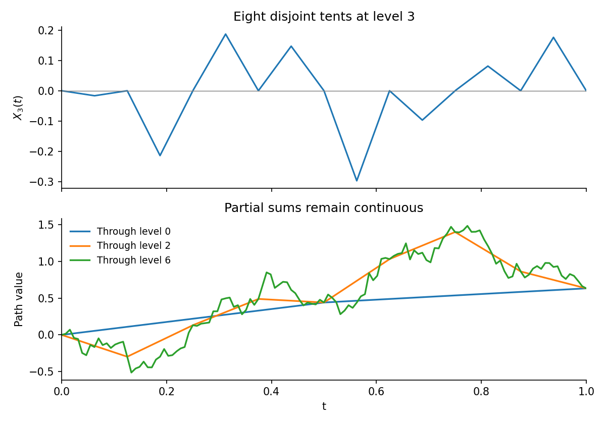
Disjoint dyadic tents and successive continuous Lévy approximations
. Details. 
The source calls a variance. Literally using that variance would give height standard deviation instead. The same maximum estimate still proves uniform convergence, since , but the resulting covariance is not that of the standard Lévy construction. The standard midpoint Brownian bridge variance on an interval of length is . Thus continuity follows under either summable scaling, while Brownian covariance requires the correct variance.
For a continuous semimartingale and a function , Itô's formula isFor Brownian motion , . With , the drift cancels:ConsequentlyThe stochastic-integral representation makes this a local martingale; localization handles unbounded . In fact it is the average of the two positive exponential Brownian martingales and , so it is a true martingale on every finite time interval.
The two-dimensional Itô formula gives the local martingale part of as , with all derivatives evaluated along . Independent Brownian coordinates have brackets and . Hence the quadratic variation isSimilarly, the quadratic covariation with isSufficient pointwise conditions are equal gradient lengths and perpendicular gradients:The Cauchy-Riemann equations , imply both. These are the quadratic covariations of an analytic Brownian image; harmonicity is needed to remove the drift, but the two bracket identities themselves follow just from the displayed derivative relations.
The solution is the continuous Doléans-Dade exponential:Here is the continuous quadratic variation starting from zero, denoted by the angle-bracket notation in the source. If with continuous of finite variation, then .
Set . Its quadratic variation is still . Applying Itô's formula to givesThe initial value is . This verification applies to the full semimartingale, including its finite-variation part.
A uniformly bounded local martingale is a true martingale: stop at a localizing sequence and use dominated convergence in its conditional-expectation identities. Its deterministic bound also gives uniform integrability. The uniformly integrable martingale convergence theorem therefore yields an integrable limit with convergence in andSince , the Radon-Nikodym derivative defines a positive measure of total mass one:The limit can vanish on a set of positive measure, so global equivalence is not required. At each finite time, however, the density is the strictly positive .
Write the integral with an explicit dummy time:On every compact time interval, strict positivity and continuity of make its reciprocal locally bounded; the covariation has locally finite variation. Thus is a well-defined continuous semimartingale.
Apply the Itô product rule. Subtracting a finite-variation process does not change covariation, so . The finite-variation terms cancel:Thus is a local martingale under .
For the transfer step, choose stopping times increasing to the horizon that bound , , reciprocal , and the brackets needed for the stochastic integrals. For each such time , the same product calculation with shows that is a true martingale. The part after is simply the bounded held value times the density martingale. By the Bayes formula for conditional expectation, for ,The stopping times exhaust the horizon also under . Hence is a continuous local martingale, proving this form of the Girsanov theorem without assuming a positive terminal density everywhere.
Articles by others on the same topic
There are currently no matching articles.