For and , is a symmetric single well. Its only minimum isThe zero is relative to the smooth background omitted from the supplied expansion.
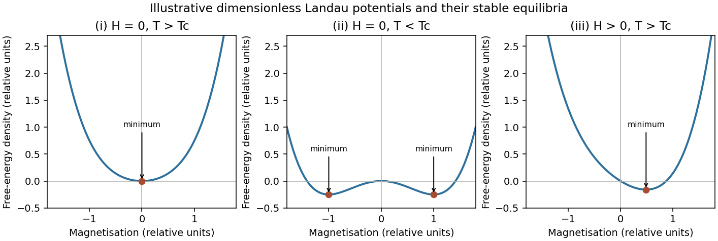
Original dimensionless quartic Landau free-energy sketches for the three printed cases, with their equilibrium minima marked
. Details. 
For and , the free energy is a symmetric double well. The central stationary point is a maximum; the two stable minima areThese are the magnetisations of the two symmetry-broken phases, selected by an infinitesimal field or a boundary condition. An exactly symmetric finite-system ensemble can have by averaging both wells; that does not make the central maximum a stable homogeneous phase.
For and , the field tilts the single well toward positive M. Since everywhere, there is exactly one minimum, at the positive solution of the equation of state. At that solution,This follows by eliminating from F. At weak field, and .
At zero applied field, time-reversal symmetry interchanges and without changing the free energy, so the analytic expansion contains only even powers. The term breaks this symmetry at fixed nonzero H. Stationarity and local stability requireFor at small field, the cubic term is higher order and . Thus the susceptibility as defined in the question isThe three requested free-energy sketches and their minima are given separately above.
For the plotted isotherms, divide the equation of state by nonzero M and rearrange:This is an Arrott plot: its slope determines b, and the isotherm through the origin identifies the mean-field Curie temperature.[ref]
Criterion for Ferromagnetism from Observations of Magnetic Isotherms by Anthony Arrott. 1957, abstract: molecular-field criterion from cubic magnetisation versus internal field at the Curie temperature
Under the paper's stated uniform-field Landau model, use H as supplied on its axis.The ordinate unit is . Reading the original graph gives slopes about – ordinate units per unit H/M, so the physical slope is approximately . ConsequentlyApproximate horizontal intercepts and the corresponding are:
The sign change brackets the transition between 19 and 25 K. A linear fit of across the four read-offs gives approximately andInterpolating only the two nearest isotherms also gives about 22 K. These are graph estimates, not exact recovered measurements.
Below at zero field, the stable branches have . Substitution gives the free-energy density relative to the omitted smooth background:The equilibrium excess heat-capacity density is below and zero above it. ThereforeThe all-isotherm linear fit gives about . Estimating the slope only between the 19 K and 25 K curves instead gives and a jump near . The lines are not exactly parallel and the intercepts are not perfectly linear in T, so a jump of order a few is supported; finer precision is not. This is per volume because F is a density; no sample volume is given to convert it to a total heat capacity.
If , the quartic truncation is unbounded below. Add a positive sixth-order term with . At zero field the coexistence conditions giveThus the zero-field transition is generically first order, with a discontinuous spontaneous magnetisation and possible metastability. It occurs before the quadratic coefficient reaches zero. The case is the tricritical boundary of this mean-field model; no value of c is invented.
Articles by others on the same topic
There are currently no matching articles.