The 2022 paper is omitted because the released copy includes worked solutions. 2022 paper with solutions, PDF pages 448–455
The fixed common temperature, rigid external container and fixed particle numbers on either side make the total Helmholtz free energy the appropriate thermodynamic potential. Let the barrier have cross-sectional area , and let increasing expand the left compartment. Then and . At fixed temperature and particle number, , soThus mechanical equilibrium, , makes stationary. The physical force on the barrier towards increasing is . If the barrier is displaced slightly from , strict mechanical stability requires a restoring force:ConsequentlyThe Taylor expansion proves that thermodynamic equilibrium is a strict local minimum of the Helmholtz free energy, rather than merely a stationary point.
For individually stable gases, the positive isothermal compressibilities make the sign especially transparent:If these inequalities hold throughout the accessible interval, is a strictly convex function and an interior stationary point is the unique global minimum of the Helmholtz free energy. Stability at one point alone proves only the local statement. A vanishing restoring derivative describes marginal stability and requires examining higher-order terms.
An additive-looking energy expression does not by itself establish two noninteracting subsystems. Their allowed microstates must also form a Cartesian product of independently available states. Here the second label's allowed values depend on the first. The four allowed pairs and their energies areThe canonical partition function, with , is thereforeThe conditional sum over is and depends on ; it cannot be pulled out as the partition function of an independent second subsystem. Summing independently over and all four values would invent four forbidden pairs and give eight states instead of four.
One can make the state labels independent by writing , but then contains a coupling between them. For genuinely additive independent energies, the difference between the and states would be independent of ; here it is . Hence the proposed and subsystems cannot be treated as noninteracting independent subsystems. The literal two-value reading of the PDF's endpoint notation has been used. If that notation were instead intended as shorthand for full angular-momentum multiplets, including every integer between the endpoints, the eight allowed states would giveThe conclusion about the failure of independent-subsystem factorization is unchanged. The two state-counting conventions should not be mixed.
A nonzero superconducting energy gap suppresses the population of thermally excited quasiparticles. When , their Boltzmann factor produces an approximately activated electronic heat capacity,where the prefactor varies algebraically rather than exponentially. For the rough estimate requested, neglect its change between the two quoted temperatures. Taking a ratio eliminates its unknown magnitude:ThereforeThe corresponding excitation energy is . The units of the two heat-capacity readings cancel in their ratio.
This is a heat-capacity activation estimate, not an exact determination of a gap from two data points. More generally, if , the same measurements giveFor example, the low-temperature BCS theory form for a fully gapped isotropic superconductor has and would give about . The stated approximate data and constant-gap assumption support the simpler estimate; they do not specify a detailed density of states or heat-capacity prefactor. Here means the minimum quasiparticle excitation energy, rather than automatically twice that value.
Put and define the thermal de Broglie wavelength of species byIgnoring the internal degrees of freedom as stipulated, each molecule's translational canonical partition function is . The two species do not interact, so their partition functions multiply; the treatment of indistinguishable particles requires a separate factorial for each species, not a factorial of the total particle number. ThusUsing and Stirling's approximation gives the extensive Helmholtz free energyThese are ideal gas expressions, valid for , with . The energy zero has been chosen so that separated CO and oxygen molecules have zero internal reference energy.
The given binding energy belongs to the formation of two carbon-dioxide molecules. Relative to the reference used in (a), the internal energy offset of one carbon-dioxide molecule is therefore , not . Its mass is and its thermal de Broglie wavelength is , where the subscript denotes .
The single-molecule canonical partition function is . For indistinguishable noninteracting molecules,The corresponding Helmholtz free energy, using Stirling's approximation, isThe negative sign in the last term expresses the stabilizing binding energy and ensures that low temperature favors association.
At fixed temperature, volume and the numbers of all other species, the chemical potential is . For the combined noninteracting mixture, add the free energies from (a) and (b). Since the thermal de Broglie wavelengths are independent of particle number at fixed temperature, differentiation givesEach logarithm has a dimensionless argument, and each chemical potential has units of energy per molecule. The binding offset must be kept consistently when comparing species.
Introduce an extent of reaction increasing in the dissociation direction. The allowed particle-number changes conserve both carbon and oxygen atoms:At fixed temperature and volume, the resulting Helmholtz free energy change isAt an interior chemical equilibrium, both forward and backward changes are allowed, so the coefficient must vanish:Equality of the three individual chemical potentials would be wrong: a reaction exchanges species in its stoichiometric proportions rather than molecule for molecule. Stability is also explicit here, sincewhen all three species are present. Thus the equilibrium composition minimizes the free energy along the conserved-composition constraint.
Substituting the chemical potentials into the equilibrium relation givesExponentiation and the positive square root give the law of mass action in number-density form:All three thermal de Broglie wavelengths have the same dependence. Define the temperature-independent mass factorIf , this exact equilibrium relation can be writtenIt already has the requested dimensional structure: has units . Its coefficient, however, depends on the conserved elemental composition through the species fractions.
For the intended case of a gas obtained by dissociating initially pure carbon dioxide, conservation of the elemental ratio gives throughout. Henceand the exact relation within this ideal-mixture model isAt high temperature with and in the dilute ideal gas regime, , this equation is self-consistently dissociation dominated:Thus , and to leading orderUsing nominal molecular masses in common mass units gives , confirming that it is of order unity. The exponential has been retained as the leading binding correction, although it tends to one as .
The printed question does not explicitly fix the elemental composition. Without the initially-pure- assumption, the universal result is the boxed mass-action relation, and approaches a composition-dependent constant when both dissociation products have nonzero high-temperature fractions. It need not be of order unity for an arbitrarily unbalanced mixture. Also, alone does not justify replacing by at arbitrarily high density; the dilute classical regime is part of the model.
A phase transition is a qualitative change of thermodynamic phase as control parameters such as temperature, pressure or chemical potential are varied. A genuine equilibrium singularity is a nonanalyticity of the appropriate thermodynamic potential in the thermodynamic limit; finite systems generally show rounded crossovers instead.
An order parameter is a macroscopic quantity that distinguishes the phases. It often vanishes in a symmetric disordered phase and becomes nonzero after spontaneous symmetry breaking, although density-driven transitions need not have that simple symmetry interpretation. It can be a scalar, vector or tensor. At a first-order phase transition an appropriate first derivative of the free energy is discontinuous, and the order parameter commonly jumps; at a continuous phase transition the order parameter can approach zero continuously while a susceptibility or a higher derivative becomes singular.
Three examples are:
- A ferromagnet below its Curie temperature has a nonzero spontaneous magnetization in zero applied magnetic field. Above the transition, the equilibrium magnetization vanishes in zero field. The direction of selects a broken-symmetry state.
- Near a liquid-gas critical point, the density contrast distinguishes the coexisting liquid and gas. It tends to zero at the critical point; below that point, changing the conjugate chemical potential through coexistence switches between low- and high-density phases.
- At an isotropic-to-nematic transition of a liquid crystal, the nematic order parameter is a symmetric traceless tensor, for example , where is a molecular orientation. It vanishes in the isotropic phase and is nonzero when the molecules preferentially align in a nematic liquid crystal.
These examples also illustrate why an order parameter must reflect the physical distinction between phases rather than merely be any quantity that changes with temperature.
For indistinguishable classical particles the canonical partition function is an integral over phase space,The factor removes overcounting under particle permutations, and makes the classical phase-space measure dimensionless. The pair potential depends only on positions, so all momentum integrations separate. The three-dimensional Gaussian integral for each particle givesThe grand canonical partition function is , where chemical potential controls the mean number of particles. ThereforeFor , the empty products and configurational integral equal one. The factor in the interaction prevents double counting of unordered particle pairs.
Write for the number of cells; this is fixed even though the particle number fluctuates. Approximate each position integral by the cell sum , evaluating the slowly varying intercell pair potential at cell centres. With the assumed single-occupancy restriction, the fixed- contribution becomesAn occupation configuration with selects an unordered set of occupied cells. There are exactly ways to assign the temporary particle labels to that set. They all have the same interaction energy, cancelling the prefactor .
Summing over all particle numbers is therefore equivalent to summing each cell occupation independently over :The activity per cell, , is dimensionless. This is a lattice gas, with each cell either empty or occupied.
The exclusion of multiple occupation is an additional physical modeling assumption, explicitly imposed by the question. Making a cell small does not by itself forbid two point particles from entering it; a repulsive core or a dilute-occupancy approximation would be needed to justify that restriction starting from a general continuum pair potential. In the remaining parts it is part of the defined cell model.
Let be the coordination number of a lattice, the number of nearest neighbours of each cell away from boundaries. Define an effective chemical potential incorporating the cell's translational entropy:Use for an unordered nearest-neighbour bond, counted once. The occupation Hamiltonian including the chemical-potential term isUnder , one bond contributesIn a regular lattice with periodic boundary conditions, the number of bonds is , and each spin occurs in linear bond terms. ThereforeThe pair sum equals one half of the ordered sum used in the paper. Consequently the effective field isThus is the Ising model partition sum, including the displayed spin-independent constant if its absolute normalization is required. Dropping that constant changes by a multiplicative factor but leaves spin probabilities and the phase-transition argument unchanged. For simple cubic cells in three dimensions, and the first term in is . Open boundaries replace by the local coordination near the surface; the stated uniform field is the bulk or periodic-lattice result.
For attractive nearest-neighbour interactions, , the transformed model is a ferromagnetic Ising model. In three dimensions and at , its infinite-volume spontaneous magnetization has two branches. As the effective field crosses zero, the equilibrium mean spin changes discontinuously from a negative value to a positive value. Since , varying the physical chemical potential crosses this same first-order phase transition.
The particle-hole-symmetric coexistence line isThe mean Ising spin is a rescaled occupation density. Writing for the physical number density,The negative-spin phase is a dilute gas and the positive-spin phase is a dense, liquid-like phase. If the spontaneous spin magnitude at coexistence is , their number densities areThus the physical order parameter is a density or occupation imbalance, not an actual magnetic moment of these particles. In a closed system with an intermediate mean density, the same transition appears as phase coexistence between the two densities. At the density contrast vanishes continuously; above , sweeping the chemical potential gives no coexistence jump. A true discontinuity requires the thermodynamic limit; a finite sum over finitely many cells remains analytic.
Let each step have length , and let be the number of right steps among independent steps. Then has a binomial distribution and the physical displacement is . Therefore , and the position probability mass isThis is zero unless is an integer, , and is even. The parity condition matters because the walk alternates between the two sublattices. If distance is measured in lattice spacings, replace by .
Normalization follows from the binomial theorem. Its first two moments provide useful checks:These are exact discrete-time statements; a smooth continuum probability density requires coarse-graining over the lattice and its parity oscillation.
The one-step master equation for the biased random walk isExpand in a Taylor series and retain the first time derivative and the first two space derivatives. Since and ,Thus the usual continuum truncation gives the requested Fokker-Planck equation,The diffusion coefficient has units , while has units of velocity. The physical drift velocity is , because the standard advection term is . A rightward bias therefore means , , and .
The approximation must be stated carefully. The truncation is a controlled diffusion limit of a weakly biased random walk when , , and , keeping and finite. It is also the spatial diffusion approximation for a continuous-time jump process with exponentially distributed waiting times of mean .
If the original fixed-step-time walk has a finite bias, its exact variance from (a) instead gives the diffusion coefficient of the Gaussian envelope about the drifting mean:One obtains the same correction by retaining in the time expansion and using the leading advection equation to replace by . The result is . In particular, a deterministic one-way walk has zero variance, as this expression requires. Thus is the usual intended first-time-derivative approximation, not an exact variance-growth coefficient at arbitrary bias. The later continuum estimates use that convention, with the fixed-time alternative identified where relevant.
For this radial random walk on a regular tree, the drawing is an infinite regular tree of degree , not a planar lattice with closed loops. The radial coordinate is the number of edges in the unique path to the root. A non-root vertex has one neighbour inward and neighbours outward, so equal probabilities for its edges giveLet be radial distance measured in edge units. For , probability arriving in shell comes from shell by an outward step or from shell by an inward step:This has precisely the same bulk master equation as the one-dimensional biased random walk, withThe outward bias is geometric: beyond the first shell, the number of vertices is , so there are more outward than inward choices even though no edge direction is dynamically preferred. is the probability summed over an entire shell, not the probability at one specified vertex; no additional shell-size factor belongs in the boxed recurrence.
The equality concerns the evolution equation away from the root, not equality to the unrestricted full-line binomial distribution at all positions. The root imposes a different boundary rule.
At the root all neighbours are in shell one, so the probability of leaving the root for that shell is one. Conversely, a walker anywhere in shell one chooses its unique rootward edge with probability . The two boundary recurrences are thereforeTogether with and , these equations determine the distribution. In particular and , which check the special root coefficient. For the original indexing, replace by and by on the right-hand sides. Summing these equations and the bulk recurrence conserves .
Farther than a few edge lengths from the root, replace the radial coordinate by a physical coordinate and smooth the master equation. It has the same constant-coefficient Fokker-Planck equation as in (b). Under the conventional first-time-derivative truncation,The radial drift is outward. For the tree is the infinite line, its radial distance is an unbiased reflected walk, and .
The root cannot absorb probability or allow negative radial distance. Write the equation as a continuity equation, using the Fokker-Planck probability currentThe appropriate continuum boundary condition is reflecting, or zero flux:It is not generally : that simpler condition is correct only when . With the finite-bias fixed-step Gaussian convention from (b), use instead; the drift sign and zero-current boundary condition are unchanged. A continuum boundary condition represents the microscopic root region after coarse-graining, rather than reproducing each discrete root probability at individual step times.
For the infinite system with outward drift, total probability remains one, but probability at a fixed distance from the root eventually decreases as the walker moves away. The question concerns this local decay, not a loss of total probability.
The independent dimensions of the continuum coefficients are and . The drift-diffusion decay time and its associated length are, up to numerical factors:Equivalently, equating the drift distance to the diffusive width of order gives this crossover scale. Rescaling and removes the dimensional coefficients from the equation.
With the conventional coefficients used in the requested continuum derivation,where the last expression suppresses the numerical factor as requested. The elementary drifted Gaussian distribution on the full line hasAt fixed , its exponential decay factor is , so an exponential e-folding time would conventionally be called , consistent with the same dimensional scale. The reflecting half-line changes the spatial form and algebraic prefactor. The substitution gives , displaying the same exponential scale for outward drift.
For , and no finite drift-induced exponential decay time exists: the probability near the root decays only algebraically. For the finite-bias, deterministic-step Gaussian envelope discussed in (b), the corresponding dimensional expression is instead . These continuum estimates are not exact return-probability decay rates for the lattice walk at arbitrary ; in particular, a diffusion approximation need not describe far-tail return events accurately at strong bias.
Use the Gibbs-Duhem equation for a homogeneous, extensive, single-component thermodynamic phase:At fixed temperature, this becomes , with number density . Separately, at fixed particle number,The chain rule along the same isothermal process in the equation of state now givesConsequentlyThis is isothermal compressibility from chemical-potential response. Since chemical potential has units of energy per particle, the right-hand side has units of volume per energy, or , as required. The derivation assumes a smooth bulk equation of state; changing the fractions of coexisting thermodynamic phases at fixed pressure needs separate treatment.
Measure single-particle energy from the lowest state and write , with . In a homogeneous system, the number of wavevector states in a thin spherical shell is proportional to . Changing variables from to gives the density of states per unit spatial volume,where is the area of the unit sphere in dimensions; an additional internal state degeneracy would multiply this expression by a constant.
The Bose-Einstein distribution has . At saturation, , the maximum excited-state number density isOnly the lower endpoint can cause divergence. There the integrand is proportional toThe improper integral converges precisely when its power exceeds . ThusWhen , the divergence is logarithmic; when , it is a power divergence. In either case the excited states can accommodate any fixed finite density at every positive temperature, so there is no bulk Bose-Einstein condensation at nonzero temperature.
For completeness, putting and using the Gamma function and Riemann zeta function givesAt fixed density , the right-hand side reaches at ; below it the excess particles occupy the lowest state, with condensate fraction . This is Bose condensation with power-law dispersion in the homogeneous thermodynamic limit. A finite vessel or a trapping potential changes the low-energy state count and must not be silently substituted for that setting.
Use the classical dilute-gas conventionso the second virial coefficient has units of volume. The Mayer f-function formula for an isotropic pair potential isOnly separations smaller than contribute. Define and substitute , so :This is the second virial coefficient of a bounded cubic repulsion. For every finite positive , , so . There is no finite positive Boyle temperature. At high temperature, expanding the exponential givesThus the intended limiting statement isAt the other extreme the classical expression tends to , the hard-exclusion value for separation . This is a check on the integral, not a claim that a real molecular gas stays classical at arbitrarily low temperature. A molar virial expansion would instead use .
Canonical probabilities. A canonical ensemble describes a system of fixed particle number and fixed external parameters such as volume, weakly coupled to a much larger thermal reservoir. They exchange energy and reach thermal equilibrium, while the reservoir's temperature stays effectively constant. The interaction energy is negligible in the state counting. The combined isolated system is described by equal probabilities for its accessible microstates.
If its total energy is , the probability of a particular system microstate is proportional to the reservoir multiplicity at . Writing that multiplicity as , expand its entropy:The large-reservoir limit suppresses the higher terms. Normalization therefore givesThe sum counts individual microstates; when grouping them by energy, their state degeneracies must be included. This is the canonical partition function.
Classical orientational heat capacity. Hold the magnetic field fixed. Orientations of the magnetic dipole moment have the solid angle measure . With , the angular partition function isChoosing a normalized angular measure would remove , with no effect on the energy derivatives. Differentiating at fixed ,The angular average is the Langevin function. Since ,This is the heat capacity of a classical magnetic dipole, in for one magnetic moment. The word specific here refers to that single moment; independent magnetic moments have times this heat capacity. At the energy is independent of orientation and , obtained by the continuous limit. At fixed nonzero , the classical low-temperature limit instead gives .
Equipartition and its proof. The equipartition theorem states that an independent quadratic term in a classical Hamiltonian, with , contributes to its mean energy. One needs a canonical measure that factors as times the measure of the remaining variables, convergence of the integrals, and vanishing boundary terms. The coordinate must not be restricted by a thermally important hard boundary or a coupled constraint.
For , integration by parts givesIntegrate over all other variables and divide by . It follows thatThe same reasoning applies to quadratic momenta among the canonical variables. It is the number of quadratic energy contributions that is counted, not an unrestricted count of coordinate labels.
Two soft orientational directions. When , the moment is concentrated near alignment. Introduce local Cartesian coordinates in the tangent plane and . To leading order,The two quadratic terms each contribute , soThis agrees with the exact angular calculation. Treating alone as one Cartesian quadratic variable would miss the measure and the second tangent direction. There are no extra rotational kinetic terms in the stipulated Hamiltonian; adding such terms would be a different model.
Quantum spin one. The spin projections are , with . Put , where is the gyromagnetic ratio. The three energies are , irrespective of the sign of . Relative to the ground state they are . Thus, with ,Differentiation, or the canonical energy fluctuation identity , givesIn the requested limit,This spin-1 paramagnet has a nondegenerate ground state and a finite spectral gap. Excitations are exponentially rare, so its heat capacity tends to zero. Classical orientational equipartition assumed a continuum of arbitrarily small excitation energies; that assumption fails when . This is a change in the accessible state spectrum, not a violation of the equipartition theorem within its classical domain.
Availability and total entropy. The reservoir changes by and . Its particle number and the system's particle number are fixed. The reservoir's first law of thermodynamics therefore givesAdd the system's entropy change. Because are constant,Thus define the availabilityAn additive constant in is immaterial; its value above the equilibrium reference is the exergy. The Second law of thermodynamics gives , hence . A stable equilibrium maximizes total entropy over the allowed variations and therefore minimizes . The environmental enter this definition even when the system has not yet reached their values. Because both thermal and mechanical exchanges are allowed, equilibrium here includes mechanical balance; equality of temperatures alone does not ensure the minimum.
Probability and curvature. For a fixed value of a macroscopic coordinate , let count the compatible system microstates. The product of the system and reservoir multiplicities isAll factors independent of enter a normalization constant, givingHere is the constrained or effective availability for this coordinate, including the multiplicity of any eliminated variables. A nonuniform coordinate measure must likewise be retained or incorporated in that effective availability.
At a stable interior minimum, and . Its Taylor expansion givesKeeping the quadratic term yields a normal distribution,This is availability curvature and equilibrium fluctuations. The quoted fluctuation formula holds at quadratic order in the Gaussian fluctuation approximation; it is not an exact identity for an arbitrary nonlinear . Higher terms can shift the mean away from its most probable value .
Bubble equilibrium. Keep the number of air molecules fixed and include the surface energy in the system's total internal energy. For constant surface tension , this contribution is , with no surface entropy under the stated approximation. Its differential isHenceIndependent thermal and volume variations give andThe air pressure is evaluated at ; since the bubble is closed it generally depends on volume, so this equation is implicit until an air equation of state is supplied. For a sphere, , , and the pressure jump becomes , the Young–Laplace equation for a single gas–liquid interface. There is no second surface as in a thin soap film.
Isothermal volume fluctuations. With the air maintained at , eliminate its entropy in favor of its Helmholtz free energy:The identity givesUsing the curvature result,These are the volume fluctuations of a closed gas bubble. Stability requires the denominator to be positive. The negative surface contribution reflects the concavity of ; gas compression supplies the positive restoring curvature. For ideal air, , and mechanical equilibrium reduces the denominator toThe units are consistent: is pressure, so has units , the units of a volume variance. Holding externally fixed while varying would remove the gas-compression term and change this stability problem; that is not the fixed-particle-number situation here.
Numerical size of the fluctuations. The volume conversion is important:Use the specified , and . ThenWith the Boltzmann constant ,Thus the fractional root mean square fluctuation and fractional variance are respectivelyThe absolute root mean square fluctuation is . The very small fractional value supports the local Gaussian fluctuation approximation. This estimate neglects exchange of dissolved air, variations of surface tension, shape fluctuations and temperature fluctuations, consistently with the prescribed fixed-number, isothermal bubble model.
Occupation and the two-dimensional Fermi energy. For an independent single-particle state, the Fermi-Dirac distribution isThe chemical potential enforces the chosen mean particle number through , including spin states in the sum. It is common to all states in particle-exchange equilibrium and must generally change with temperature or field when the total mean number is held fixed. At zero temperature, the distribution becomes a Heaviside step function at the Fermi energy.
Let the sample area be and let be its internal spin spin degeneracy. In the continuum limit, filling the disk givesThereforeFor spin-half fermions with both spin states available, and ; for a spin-polarized gas . The question does not specify the area or spin degeneracy, so these conventions must be stated rather than extracting an energy from alone. Although the original text calls momentum, the supplied dispersion makes it a wave vector; physical momentum is . The result agrees with the constant two-dimensional free-electron density of states. Discrete level spacings in a finite sample would require a specified boundary spectrum.
One level occupied on average. Write and . The two mean spin occupations areImposing gives , hence . Thus, for every positive temperature,The total magnetic moment is . ConsequentlyThis is the grand-canonical spin susceptibility of a half-filled single level. Empty, singly occupied and doubly occupied orbital states are allowed in the grand canonical ensemble. At zero field, the singly occupied configurations together have probability , explaining the factor of two relative to one permanent spin-half moment. If exactly one Electron were required at all times, a canonical two-state partition function would instead give and . That different answer does not implement the stated average-number constraint.
Density-of-states formula for the susceptibility. Here is the zero-field single-spin density of states. Regard its argument as the full spin-shifted energy. The shifted functions are , soThe total number is even in ; thus at fixed total number on a smooth branch. More directly, terms from cancel in the spin difference because the two densities coincide at zero field. To first order,It follows thatFor a physical energy band, take to vanish below its lower edge. Provided the endpoint term vanishes, integration by parts also givesThis form displays the positive response and the narrow thermal window around . A sharp band edge is included by the corresponding distributional derivative in the first expression. The susceptibility defined here is the derivative of total magnetic moment with respect to , with units ; it is not automatically a dimensionless SI volume susceptibility. A density-of-states convention per unit volume likewise gives a response per unit volume. These are the field conventions for magnetic susceptibility.
Chemical potential at fixed number. Define the integrated single-spin state countThe probability kernel has unit integral, mean , and variance . Using integration by parts,Expand about . The linear term integrates to zero, while givesThis is the number form of the Sommerfeld expansion. Since at zero temperature, set with :ThereforeThe coefficient can be obtained directly. With ,For example, the sum follows by expanding on , using the evenness of the kernel and integrating each exponential. Thus . A density of states increasing with energy gives a downward quadratic chemical-potential shift. For the constant two-dimensional density of states that shift vanishes to this order; a finite lower band edge still allows exponentially small corrections.
Low-temperature susceptibility at fixed number. Apply the same kernel expansion to itself:The shift of must be retained in the first term. Writing and similarly for its derivatives,ConsequentlyThis is the fixed-number low-temperature Pauli susceptibility. The contribution is thermal broadening at fixed chemical potential; the contribution enforces fixed total number. Both are needed. If the density of states were instead defined with both spin directions included, the prefactor would be absorbed into that definition. Only the spin response has been calculated; no orbital magnetic response is included.
The expansion assumes , sufficient smoothness near the Fermi energy, and a temperature small compared with the energy scale over which changes or encounters a band edge. It does not apply unmodified at a singular density of states. For the ideal two-dimensional parabolic band, , so the leading Pauli response is temperature independent, consistently with the earlier state count.
First solve the equation of state for the volume:The Gibbs free energy has differential . At fixed temperature and particle number, integrate between the two pressures:ConsequentlyUse , keeping both endpoint pressures fixed while differentiating the difference:Equivalently, the Maxwell relation gives , whose pressure integral is the same result. These are the Gibbs free-energy change for a pressure-linear gas correction identities. The physical path requires and positive volume throughout. The correction has units of volume per particle, so each term in is an energy and each term in has units of energy per kelvin.
For a phonon mode of angular frequency , the equilibrium occupation isWell above the Debye temperature, the relevant vibrational energies are small compared with . Expanding the exponential givesThe spectrum and its cutoff are fixed in the model, so the remaining sum is temperature independent. ThusFor example, the three-dimensional Debye model with gives . This is the high-temperature phonon number in the Debye model. The number of phonon quanta can exceed ; counts modes, not their total occupation. Under the stipulated proportionality to phonon number, only the phonon contribution to resistivity has been calculated. A temperature-independent residual resistivity would add an intercept in a real sample.
Particles within each species are indistinguishable, while the two species are physically distinguishable and their numbers are fixed. Independence makes the canonical partition function factor by species:Since at fixed volume, . The canonical entropy is thereforeFor large species populations, Stirling's approximation gives the equivalent Sackur-Tetrode equation formFor structureless particles with the same translational partition function, , where is their common thermal de Broglie wavelength. More generally the supplied common constant factor in should be retained in the entropy.
Writing separates the total-number contribution from the composition term:The last term is the entropy of mixing relative to separated ideal components at the same temperature and pressure. This is the entropy of a two-species classical ideal gas. Artificially labeling otherwise identical chemical atoms would not justify dividing by separate factorials or adding a mixing entropy. The pure-species limit is obtained by .
Fermion occupation and ordinary metallic heat capacity. The Fermi-Dirac distribution for a single-particle state isAt low temperature it changes appreciably only in an energy window of width of order about . If the full density of states is smooth and nonzero there, only about states change population. Each excited particle or hole carries energy of order relative to the Fermi surface, so is of order . Differentiation therefore gives .
More precisely, the fixed-number Sommerfeld expansion givesHere includes all counted internal species. This argument requires and a density of states varying slowly across the thermal window; a band edge or vanishing density of states can change the power law.
Two-dimensional linear dispersion at zero chemical potential. Let count identical positive-energy branches, keeping the state-counting convention explicit. The number of wavevector states in a ring of radius is . With , this givesAt , the thermal energy of this branch isThe dimensionless integral is . Differentiating givesThis is the heat capacity for a two-dimensional linear fermion dispersion. A physical neutral particle–hole-symmetric Dirac cone also has electron holes in its filled negative-energy band. Their excitation energy gives an equal contribution, doubling for the same cone count. The scaling is unchanged. For a positive-energy-only gas, holding allows its mean particle number to vary; a neutral two-band surface instead maintains zero net excess charge as Electron–hole pairs are thermally excited. These conventions should not be conflated when specifying an exact coefficient.
Nonzero chemical potential. The ordinary metallic regime isThe thermal window then lies far from the cone tip. Since , its fractional change across that window is only of order . Treating it as locally constant restores the Sommerfeld result . When is comparable to or larger than , the window probes the vanishing density of states near the tip and crosses toward the neutral behavior, provided the linear dispersion remains valid.
Bulk phonons and the surface-to-bulk comparison. For the topological insulator model, assume bulk electronic excitations are frozen out while the conducting surface remains active. In three dimensions, acoustic phonons have a density of modes proportional to . Normalize the Debye spectrum to modes:The thermal part of the energy isAt , extending the upper integration limit to infinity introduces an exponentially small error. With and ,Temperature-independent zero-point energy makes no contribution to this heat capacity. The requested ratio consequently scales asFor a fixed shape and composition, and , so the ratio grows as . Smaller samples and lower temperatures favor the surface contribution. It dominates if the dimensionless right-hand side, including its state-counting prefactor, exceeds unity. This is the surface-electron and bulk-phonon heat-capacity crossover.
The continuum electronic law also requires a thermal energy larger than the surface finite-size level spacing, of order . The phonon continuum has its own finite-size cutoff. Therefore dominance obtained by formally taking cannot always be inferred from the two continuum power laws alone.
There is a numerical-normalization qualification in the paper. Combining the explicit one-positive-branch result above with the conventional -mode Debye normalization gives ratio prefactor ; including electron holes doubles it. For , this is approximately before that doubling, rather than the supplied . The problem specifies neither a cone/spin multiplicity that equates these nor another mode normalization. Its supplied prefactor is therefore used as the stipulated approximation for the requested numerical estimate, rather than claimed as an exact consequence of the single-branch count.
Numerical estimate. A cubic sample of volume has side . Counting the conducting surface on all six faces givesFor one atom per cubic cell of side ,Use and . Inserting the stated , and into the paper's supplied prefactor givesThus bulk phonons dominate at this temperature in this estimate. If only one face contributes, the ratio is ; if there are chemical atoms per unit cell, divide the corresponding estimate by . These geometrical and crystallographic factors are not supplied explicitly.
With the same prefactor and geometry, extrapolating would suggest equality near . However, the surface finite-size scale is already of order for this specimen. That extrapolated crossover lies outside the continuum electronic regime, so it is not a reliable prediction of the sample's ultimate lowest-temperature heat capacity.
Classical translational statistics. Write the number density as and the thermal de Broglie wavelength as . Quantum exchange is negligible when wave packets rarely overlap:The equivalent state-counting statement is that the mean occupation of each thermally relevant one-particle state is much smaller than one. The equations in this question count one internal species; with equally populated spin states the relevant density per species is .
Let be the dimensionless quantum gas fugacity, with the lowest one-particle energy chosen as zero. Both quantum distributions can be writtenIf , then for all , recovering Maxwell–Boltzmann statistics. Conversely, low occupation even at the spectrum's bottom requires for bosons or for fermions; either condition impliesA single high-energy state can be sparsely occupied even in a degenerate gas, so the condition must hold across the relevant spectrum, not just for one arbitrarily chosen energy. Also, classical translational statistics does not imply that all internal excitation energies or other quantum effects can be ignored.
Grand partition function, density and pressure. Noninteracting particles have independent occupations of each one-particle state. Put . Summing the allowed occupations givesThereforeThe grand potential is for this homogeneous gas. Replacing the sum by and using givesThe mean number is , givingFor bosons, the grand sum requires when the ground energy is zero. A macroscopic condensate at the limiting must be separated from the continuum integral in the condensed phase. The following small- calculation is in the normal, nondegenerate regime, so that complication does not enter.
Density expansion and inversion. Expand the occupation as a geometric series:The Gaussian wavevector integral for its th term isIt follows thatFor the inverse series, put and try . Substitution gives , henceThe leading equality directly connects the density and occupancy criteria for classical behavior.
Pressure and its first quantum correction. Expanding the logarithm in the pressure expression gives one extra factor compared with the density series:Insert the inverse series. To second order in ,ThusThe first quantum correction at fixed density and temperature isIt is negative for bosons and positive for fermions, and vanishes in the classical density limit.
Virial coefficient. Define the number-density virial expansion byThe coefficient has units in this convention. Comparing terms givesThis is the exchange contribution to the second virial coefficient. It arises without a pair-interaction potential; the underlying gas is noninteracting. A molar-density convention would multiply this by the Avogadro constant. For equally populated internal species, exchange occurs within each species and the coefficient in terms of total density is smaller by a factor .
Why the two signs differ. Bosonic exchange symmetry enhances the probability of nearby identical bosons, whereas fermionic exchange symmetry suppresses nearby identical fermions in the same internal state. In the dilute regime, the normalized equal-time pair detection correlation isThe exchange part follows by squaring the Gaussian one-particle coherence factor . At zero separation this gives for bosons and for one-component fermions. Integrating the exchange pair weight provides a direct coefficient check:Bunching therefore acts like an effective statistical attraction in the dilute equation of state, lowering the pressure needed at fixed density. Exclusion acts like an effective statistical repulsion, raising it. Neither description asserts an actual interparticle force. Different internal fermion species do not exclude each other from a common spatial location in the same way, explaining the importance of the species convention.
Order parameter and the free-energy landscape. In Landau theory, take a scalar magnetization component at fixed volume and composition. It is an order parameter: its nonzero spontaneous value distinguishes an ordered phase with ferromagnetism from the symmetric high-temperature phase. One first constructs a constrained order-parameter free energy at specified magnetization by summing over microscopic states compatible with it. An external magnetic field is an independent control, so it can also appear in that constrained function. For a total magnetic moment the conjugate term is ; if is a magnetization density, the total-energy term is , or in free-energy density. Minimizing over then yields the equilibrium thermodynamic potential as a function of the imposed field.
Thus treating both and as arguments of a Landau function does not treat them as independent natural variables of the already-minimized equilibrium free energy. The first is the fluctuating or constrained order parameter, and the second its conjugate field.
At zero field, reversal symmetry requires , excluding odd powers. Near a continuous transition, assume the homogeneous constrained free energy is analytic for small , that the quadratic coefficient crosses zero linearly, and that the quartic coefficient is positive. ThenThe temperature is where the zero-field quadratic coefficient vanishes and spontaneous ordering begins in this approximation. Higher powers are negligible sufficiently close to it; spatial fluctuations are neglected in this mean-field treatment.
Stationarity gives . Above , the only minimum is at zero. Below it, zero becomes a maximum and two minima appear:The two signs describe spontaneous symmetry breaking: they are the average magnetizations in the symmetry-broken pure phases. A strictly finite system at exactly zero field samples the two wells symmetrically and has ensemble average . A spontaneous pure-phase value is defined by selecting a phase, for example taking the thermodynamic limit before removing a small field. This qualification distinguishes a minimum's location from the average over a symmetric two-well distribution.
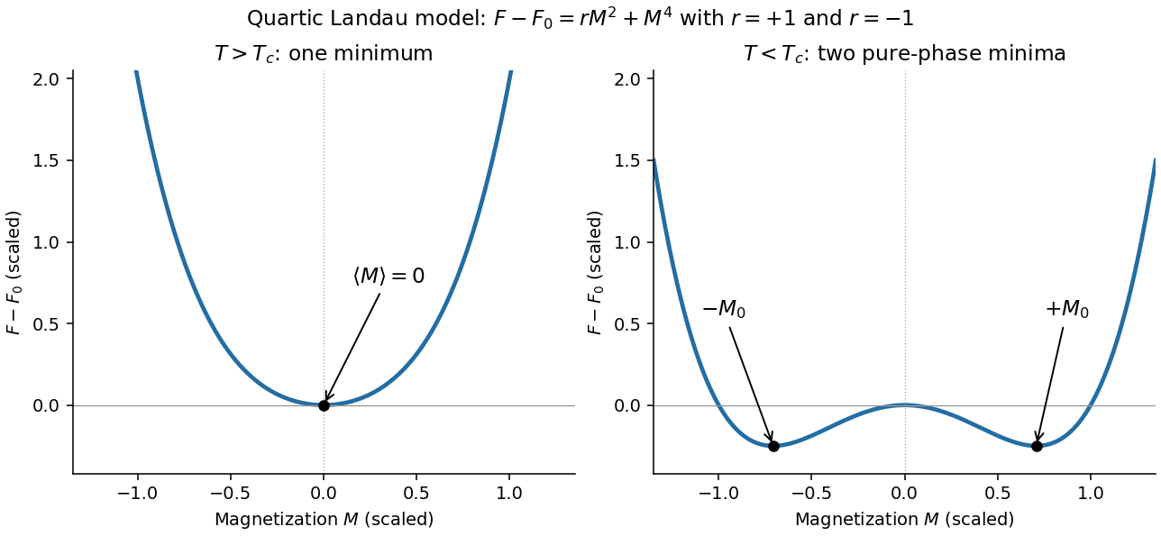
Quartic Landau free energy above and below the transition, showing the disordered and symmetry-broken minima
. Details. 
Minimum free energy and the heat-capacity jump. At a nonzero minimum, . Substituting this value givesHencewhile above the transition. Take the temperature derivatives only after minimizing, so the equilibrium order parameter is allowed to change with temperature. With ,ThereforeThis is the heat-capacity jump in quartic Landau theory. The entropy is continuous at , so there is no latent heat. If denotes free-energy density rather than total free energy, these expressions denote heat capacity per unit volume with the same normalization.
Stabilizing a tricritical expansion. At a tricritical point, the quartic coefficient is tuned to zero at the same point where the quadratic coefficient changes sign. Reversal symmetry still excludes odd powers. The next available stabilizing term is thereforeA negative or vanishing leading sextic coefficient would not stabilize this truncation for large ; a higher positive term would then be needed and the present tricritical form would be insufficient. The ordinary quartic theory has a continuous transition for , while a stabilized theory with can have a first-order transition. Their meeting at zero field is what makes the simultaneous tuning tricritical.
The tricritical minimum. At zero field and , stationarity givesThe nonzero solutions are minima: their curvature is . Put . Since at stationarity,ThusThe order parameter now vanishes as rather than the quartic theory's square root.
Heat-capacity singularity. Define , so the ordered-side singular free energy is . Its derivatives areConsequentlyThis is the tricritical heat-capacity amplitude in a sextic Landau expansion. It is positive on the ordered side and diverges as , rather than remaining a finite jump. This value of the heat-capacity critical exponent is the mean-field result along the path keeping the quartic term zero; a detuning to ultimately restores ordinary quartic behavior. Fluctuation corrections to the mean-field theory are not included in the stipulated polynomial minimization.
Put and . The BCS quasiparticle spectrum has , so on either inverse branchConservation of states on one branch gives . Consequently the single-branch expression requested in the source isThere are no such states for in this ideal fully gapped model. Near the edge the density of states diverges as , an integrable singularity; at large it approaches its normal-state value.
Counting qualification. The energy map in the source is two-to-one. If literally counts all normal-state levels both above and below , the unweighted positive-energy quasiparticle density from a folded spectrum must sum both preimages, and is insteadAlready at , folding into doubles the positive-axis density. Thus the printed formula is not the unweighted count of all states under the literal mapping without an additional normalization convention.
There is also a standard physical quantity with exactly the printed normalization: the BCS electronic density of states, measured for example by single-electron superconducting tunneling. At positive , the electron spectral weights of the two roots are the BCS coherence factors . They sum to one, so the weighted sum is . This supplies a valid electronic-DOS interpretation, while keeping it distinct from counting every positive-energy excitation. Spin degeneracy must be included consistently in and the transformed density; it does not remove the branch-counting issue.
Repeated letters. There are six positions, with two copies of each of two letters. Counting labeled arrangements and dividing by the permutations of each repeated pair gives
Single-occupancy cells. For indistinguishable particles, specifying which of the distinct cells are occupied completely specifies a configuration. ThusFor distinguishable particles, each chosen occupied set admits assignments of particle labels:Equivalently, successively place labeled particles in available cells. The single-occupancy constraint is essential: this is not unrestricted stars and bars. Both counts give one empty configuration at ; at they give one unlabeled occupation pattern and labeled assignments.
In the grand canonical ensemble, the system exchanges both energy and particles with a reservoir at fixed temperature and chemical potential . The probability of a particular many-body microstate , with energy and particle number , is its Boltzmann weight divided by the grand canonical partition function , where . The denominator normalizes ; a degeneracy is accounted for by counting distinct microstates, rather than changing an individual state's probability.
For noninteracting particles, specify a microstate by the occupation numbers of one-particle levels of energy . Then , so the Gibbs probability factorizes between levels. Put .
For fermions, the Pauli exclusion principle permits in each complete one-particle state, giving . Its mean occupancy isthe Fermi-Dirac distribution.
For bosons, , so the geometric sum is when . Differentiating that sum givesthe Bose-Einstein distribution. Finite-system convergence requires ; condensation is the limiting approach to the lowest energy with macroscopic ground-state occupation. Both quantum distributions reduce to when occupation is small. The quantities derived here are mean occupancies of states, rather than normalized probabilities over the set of one-particle energies.
Structure through pair correlations. For a homogeneous isotropic monatomic liquid of number density , the radial distribution function is defined byIt compares the conditional density around a tagged particle with the bulk density. A repulsive core makes close neighbours unlikely; a first peak identifies a preferred coordination shell, and damped peaks at larger radii describe short-range order. Far away, in the bulk limit. Unlike a crystal, an ordinary liquid has no indefinitely repeated positional order. An ideal uncorrelated gas has away from the tagged particle. The shell factor must not be confused with itself.
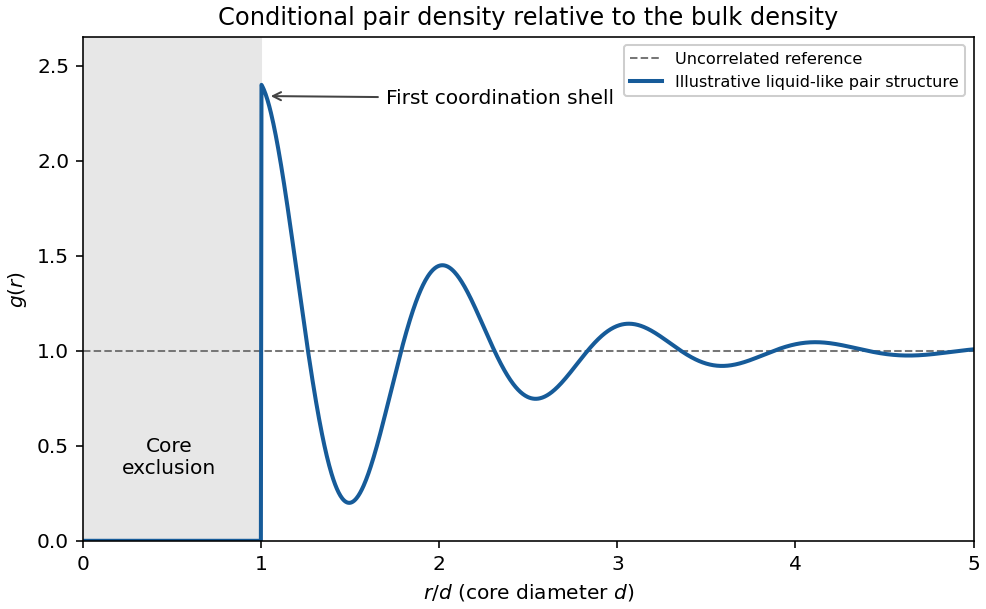
Original schematic radial distribution function showing a core exclusion region and damped liquid-like coordination shells; the curve is illustrative rather than measured data
. Details. 
The same pair structure enters the static structure factor measured through scattering. In the bulk isotropic convention,Thus real-space coordination and reciprocal-space scattering peaks describe the same correlations.
Energy from the structure. If interactions are sums of a central pair potential , the equipartition theorem gives the classical kinetic energy . Count the interaction of a tagged particle with its neighbours and divide by two to avoid counting each pair twice. The pair-correlation expression for internal energy isThis makes structure thermodynamically useful: short-distance repulsion and the attractive region contribute with different weights. Additional internal molecular modes or many-body interactions require extra terms. The formula is a classical bulk pair-potential result, not a universal energy formula for every liquid.
Pressure and the dilute expansion. The mechanical virial theorem relates the pair forces to pressure. The virial pressure from pair correlations isAt low density, , giving the virial expansionThe second virial coefficient has units of volume per particle; higher coefficients encode additional cluster correlations. A hard-sphere exclusion diameter gives . Attractions contribute negative terms and can make negative. Although the pair-correlation formulas can describe a dense liquid when its actual is known, truncating the virial series after a few terms is normally a dilute-fluid approximation. It should not be silently extrapolated through condensation or into a dense liquid.
Excited-state saturation. Consider first a uniform three-dimensional noninteracting gas of identical spinless bosons in a large box. Set the one-particle ground energy to zero. The Bose-Einstein distribution is , with quantum gas fugacity . For dispersion , the excited density of states isUsing the thermal de Broglie wavelength , integration givesThe polylogarithm is . Its finite value at implies a maximum excited population , with . Once this is less than , the excess particles occupy the ground state macroscopically. This is Bose-Einstein condensation, rather than occupation of a state by merely one or a few atoms.
Transition and condensate fraction. Setting the saturation number equal to gives the homogeneous ideal Bose gas condensation temperatureBelow this temperature, approaches zero from below in the thermodynamic limit, and particle conservation givesAbove there is no macroscopic condensate and adjusts to keep fixed. At finite , the chemical potential remains slightly below the ground energy and the transition is rounded.
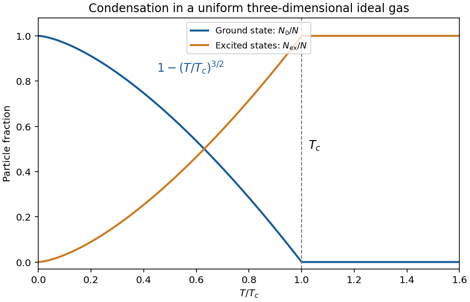
Original uniform ideal-gas condensate fraction and schematic accumulation in the lowest state below the critical temperature; the exponent is for a three-dimensional box
. Details. 
Energy and the role of geometry. The excited-state internal energy isThe zero-energy condensate contributes no term to this energy in the ideal model. Below ,Condensation depends on low-energy state counting: for a uniform quadratic-dispersion gas, a finite-temperature bulk condensate requires spatial dimension greater than two. A trap changes the density of states and therefore the temperature law; a three-dimensional harmonic trap gives a cubic, rather than , condensate-fraction exponent. Finally, an ideal-gas condensate should not automatically be called a superfluid: its free quadratic spectrum has zero critical speed by the Landau criterion. Interactions matter for the robust collective-flow properties of real dilute condensates.
Quanta of collective motion. An elementary excitation is a low-energy departure from the many-body ground state that can often be treated as a quasiparticle. Near an ordered equilibrium, small collective motions form normal modes. Quantization turns a harmonic mode of frequency into bosonic excitations with energy . Their number is not an independently conserved thermodynamic variable in equilibrium, so their chemical potential is zero andHere labels branches, and contains the ground-state contribution, including phonon zero-point energy where appropriate. The approximation is useful while interactions and damping of the excitations are weak enough that the modes remain identifiable.
Phonons. A phonon is a quantum of an elastic lattice-vibration mode. Long-wavelength acoustic phonon branches have , with one longitudinal and two transverse polarizations in a three-dimensional monatomic solid. A multi-atom primitive cell can also support optical phonon branches, generally with nonzero frequency at . Linear acoustic dispersion gives , so the energy integral has and the heat capacity obeys the Debye law. In the Debye model,At temperatures high compared with all phonon energies but below structural changes, the classical harmonic limit gives approximately . Optical modes are frozen out at temperatures well below their gaps.
Spin waves. A spin wave is a spatially varying collective precession of ordered spins; its quantum is a magnon. In a simple isotropic ferromagnet, a long-wavelength gapless branch has energy , where the spin stiffness has units . State counting gives . For one isotropic branch in three dimensions,This exponent is specific to a gapless quadratic ferromagnetic branch. Long-wavelength antiferromagnetic spin waves can be linear and instead give a heat-capacity law in three dimensions. Magnetic anisotropy or an applied field can open a gap, causing activated behaviour at still lower temperatures. Near a magnetic ordering transition, a dilute noninteracting spin-wave description is no longer adequate.
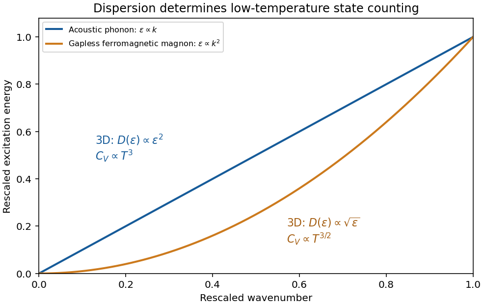
Original schematic linear acoustic-phonon and quadratic ferromagnetic-magnon dispersions with their three-dimensional low-temperature heat-capacity powers
. Details. 
These examples illustrate the low-temperature energy of gapless bosonic excitations: for in dimensions, , hence and . The exponent records both the spatial dimension and the dispersion, making calorimetry a probe of elementary excitations.
Component chemical potentials. Define the per-spin quantum concentration . For a classical component with one-particle potential energy , the local Helmholtz free energy density is . Its derivative with respect to number density gives the full local chemical potential, including the magnetic energy. With the up state defined as the lower level,The Bohr magneton is a magnetic moment; is an energy. The factor two for the two spin states is not already included in .
Total equilibrium chemical potential. If spin conversion is allowed, a particle can be added in either spin state at the same equilibrium free-energy cost. Thusnot their sum or zero. The total particle number, or a reservoir, fixes this common value; the supplied information does not specify a numerical chemical potential. A useful local expression is , with , whose density dependence is found below.
Why it is uniform and common. Moving a small number of one species from to changes the free energy by . If this difference were nonzero, a transfer could lower the free energy. Equilibrium under diffusion therefore requires each full chemical potential to be spatially constant. A spin flip transferring from down to up similarly changes free energy by , proving equality when spin relaxation is permitted. This is chemical equilibrium of a classical spin gas. Mere thermal contact at fixed separate spin populations would not enforce the latter equality; full spin equilibrium is the necessary assumption. A spatially varying magnetic field is balanced by a spatially varying density, not by a varying full chemical potential.
Magnetization. Invert the component equations at the common :The two levels have moments and along the field. The magnetization, magnetic moment per unit volume, is thereforeIts SI units are . This expression neglects interactions and magnetic feedback of the gas on the specified external field.
High-temperature response. For , and , yieldingAt fixed number density, this is the Curie law: the susceptibility with respect to is . The conventional dimensionless susceptibility with respect to is approximately when . At fixed , however, changes with temperature, so itself need not scale simply as . The moment per particle has the Curie behaviour; the density constraint must be stated.
Total density. Adding the two populations givesFor a finite container and fixed , normalization gives . In a weak field the leading density is uniform, with changes only of order . Particles preferentially occupy regions where the magnitude of the field lowers one of the spin energies, even though the common chemical potential remains uniform.
Gibbs free energy and its minimum. For fixed atom number , there are sites andconfigurations with indistinguishable vacancies. Their configurational entropy is . Relative to the vacancy-free Gibbs free energy , creating vacancies costs energy and pressure-volume work . Put . ThenAt leading thermodynamic order, Stirling's approximation givesThe minimum obtained from the stationary point below isIf the perfect crystal's internal energy and other entropy are chosen as zero, its pressure term is . More generally the information given fixes the vacancy contribution rather than the absolute bulk free energy. The pressure-volume term must be retained because the number of sites, and hence the volume, changes.
Equilibrium vacancy population. Differentiating the extensive free energy at fixed givesThe stationary point is consequently the unique interior minimum. Write ; its condition is , giving the requested thermodynamic result for equilibrium vacancies with variable lattice size,Substitution back into cancels the terms containing and yields the boxed minimum. In the dilute-defect limit , . The Bose-like denominator is a consequence of the changing number of lattice sites and combinatorial entropy; it does not assert that vacancies here are an ideal gas of bosonic particles.
There is a finite-size correction to a variable-site vacancy model if “average” is interpreted exactly. The microscopic count written above gives the relative isothermal-isobaric sumsoIts relative equilibrium free energy is . Thus the source's numerator is correct to leading extensive order, but is not the exact finite- mean for that stated configuration count. A free-energy minimum is likewise not generally identical to the mean of a finite distribution. These distinctions vanish relatively as .
Thermal volume. Each atom or vacancy occupies volume , so at the same thermodynamic accuracyFor the exact counting model, replace by in . The vacancy-free limit is as . This model isolates expansion from vacancies, taking and constant; it omits ordinary phonon thermal expansion. Its growth at high temperature should not be extrapolated to arbitrarily large vacancy fractions in a stable crystal, and is essential for a normalizable variable-site ensemble.
One particle. Use the classical phase-space normalization of one quantum state per volume , with no unspecified internal degeneracy. For and , the canonical partition function factorizes into momentum and position integrals:The Gaussian momentum integral is . In spherical coordinates, put :Therefore the classical ideal gas in a spherical linear trap hasHere is a force, in , so is a length and is dimensionless. A nonconfining would not give this finite spatial integral. As required by the classical phase-space approximation, the temperature must exceed the trap's discrete level scale.
Indistinguishable dilute particles. Independent labeled particles would give . In the classical dilute regime, division by removes the overcounting of permutations of identical particles:This is the Maxwell-Boltzmann limit, not an exact quantum canonical partition function at high occupation. Exchange effects cannot be captured merely by continuing this formula beyond its dilute regime.
Free energy, energy and entropy. The Helmholtz free energy isWith leading Stirling's approximation, , this becomesAt fixed trap strength, . Differentiating gives the requested entropy,The is : the first term comes from indistinguishability through Stirling's formula, and the second from the temperature dependence of . Without the large- approximation, . Independently,The kinetic contribution is and the linear-trap potential contribution is , also obtained from generalized equipartition.
Entropy curves and reversible cooling. For a fixed and a reference pair , the dependence can be written without logarithms of dimensional quantities:At each fixed , the entropy increases logarithmically and is concave downward in ; decreasing shifts the curve upward. Its formal classical divergence as marks failure of classical statistics, not a physical negative-infinite entropy.
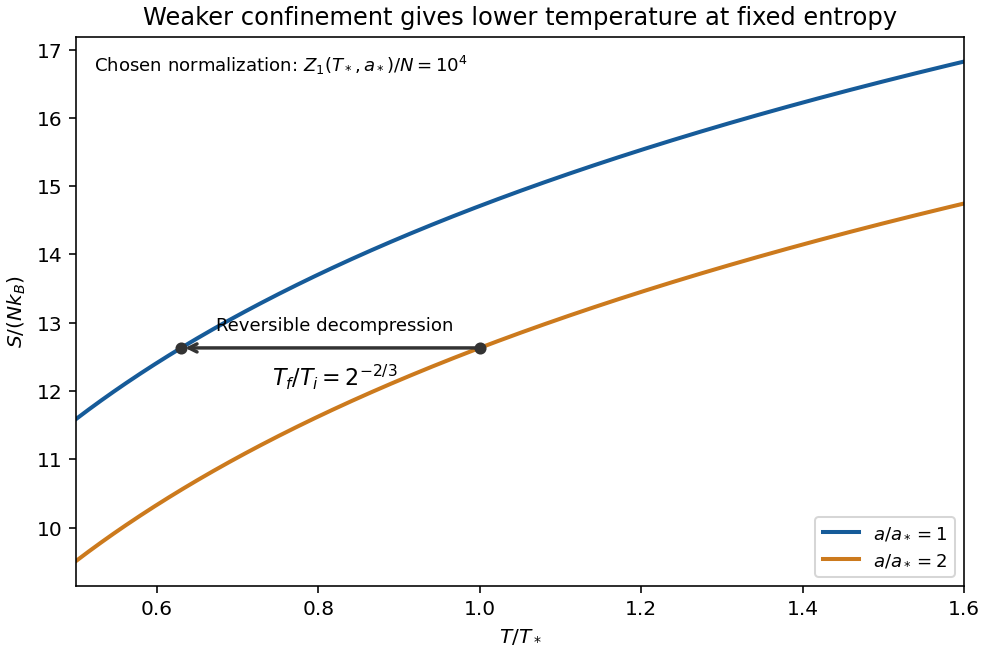
Original classical entropy curves for two linear-trap strengths; a horizontal constant-entropy arrow shows cooling on reversible decompression, within the dilute regime
. Details. 
For a reversible adiabatic change, is constant at fixed , soHence reducing lowers the temperature: this is isentropic decompression of a spherical linear trap. The gas does work on the control that weakens the trap. Equivalently , with ; inserting gives the same relation. Reversibility requires an equilibrium sequence without heat input or entropy production. Because stays constant on this adiabat, also stays constant: this mechanism cools the cloud but does not by itself increase quantum degeneracy.
Chemical potential and quantum threshold. From the extensive free energy,Thus the quantum gas fugacity is . Classical statistics requires ; quantum effects become important as the chemical potential comes within order of the lowest one-particle energy. With the semiclassical zero at the potential minimum, the quantum degeneracy threshold in a spherical linear trap is consequentlyThere are no numerical values of in the paper, so this parameter-dependent estimate is the requested atom number. It also follows from the peak density: , and degeneracy starts when is order one. The criterion is a crossover estimate, not an assertion that the classical formula remains valid at . For spinless bosons the continuum excited-state saturation is more specifically , while for fermions the onset is occupation constrained by exclusion. At temperatures comparable with the quantum trap spacing, the actual ground energy must be included consistently rather than identified exactly with the classical minimum.
Articles by others on the same topic
There are currently no matching articles.