Past exam of the year 1 of the computer science course of the University of Oxford / 2017 / Imperative programming (resit) (A10098W1)

Solutions to the 11 September 2017 resit, with all 35 printed subparts answered. Source: released examination archive, member a10098w1-1.pdf.

The first section uses Oberon-style procedure fragments and algorithmic pseudocode; the second uses the Scala 2 syntax of the paper. Arithmetic-operation counts assume exact integer operations, with arbitrary-precision bit costs considered separately.

1

a

Solution

Use the supplied pointer-to-record representation and allocate a fresh record:

PROCEDURE mkRat(n,d: INTEGER): rational;
VAR z: rational;
BEGIN
  ASSERT(d # 0);
  NEW(z); z.num := n; z.den := d;
  reduce(z);
  RETURN z
END mkRat;

The rational number constructor returns a value with positive denominator in lowest terms, using part (b). Zero is represented as

0/1

. Arithmetic below uses exact integers, or inputs whose intermediate values fit the chosen implementation; fixed-width overflow would otherwise invalidate exact arithmetic.

b

Solution

Divide numerator and denominator by their positive greatest common divisor, then fix the sign:

PROCEDURE reduce(x: rational);
VAR g: INTEGER;
BEGIN
  ASSERT(x.den # 0);
  g := gcd(ABS(x.num),ABS(x.den));
  x.num := x.num DIV g; x.den := x.den DIV g;
  IF x.den < 0 THEN
    x.num := -x.num; x.den := -x.den
  END
END reduce;

The denominator condition ensures

g > 0

, including when the numerator is zero. Dividing both components by the same nonzero integer preserves the fraction, and the final simultaneous sign change preserves it again. The resulting numerator and denominator are coprime; for zero the denominator becomes one.

c

Solution

Use the ordinary fraction identities, returning fresh records rather than changing either argument:

PROCEDURE addRat(x,y: rational): rational;
BEGIN
  RETURN mkRat(x.num*y.den + y.num*x.den, x.den*y.den)
END addRat;

PROCEDURE mulRat(x,y: rational): rational;
BEGIN
  RETURN mkRat(x.num*y.num, x.den*y.den)
END mulRat;

PROCEDURE negRat(x: rational): rational;
BEGIN
  RETURN mkRat(-x.num,x.den)
END negRat;

Every result is reduced by mkRat. This preserves the representation invariant even if an input was initially unreduced, provided its denominator is nonzero. Aliasing between the arguments causes no problem because their fields are only read.

d

Solution

Represent

a + b 5

by the pair

(a, b)

in the quadratic field

Q (5)

. Its multiplication rule is

(a + b 5) (c + d 5) = (a c + 5 b d) + (a d + b c) 5 .

The constructor copies both rational components, so later reduction through another pointer cannot change the constructed value:

PROCEDURE mkIrr(r,i: rational): irrational;
VAR z: irrational;
BEGIN
  NEW(z);
  z.rat := mkRat(r.num,r.den);
  z.irr := mkRat(i.num,i.den);
  RETURN z
END mkIrr;

PROCEDURE addIrr(x,y: irrational): irrational;
BEGIN
  RETURN mkIrr(addRat(x.rat,y.rat),addRat(x.irr,y.irr))
END addIrr;

PROCEDURE mulIrr(x,y: irrational): irrational;
VAR r,i: rational;
BEGIN
  r := addRat(mulRat(x.rat,y.rat),
              mulRat(mkRat(5,1),mulRat(x.irr,y.irr)));
  i := addRat(mulRat(x.rat,y.irr),mulRat(x.irr,y.rat));
  RETURN mkIrr(r,i)
END mulIrr;

The representation includes rational values when the second coefficient is zero; the supplied type name does not require every stored value to be irrational.

e

Solution

First normalize fresh copies of the two components. The following output helpers print a reduced rational with no /1, suppress a zero radical term, and suppress a unit radical coefficient:

OutRat(q):
    Out.Int(q.num)
    if q.den != 1: Out.String("/"); Out.Int(q.den)

OutIrr(x):
    r = mkRat(x.rat.num,x.rat.den)
    b = mkRat(x.irr.num,x.irr.den)
    if b.num == 0:
        OutRat(r); return
    if r.num != 0: OutRat(r)
    if b.num < 0: Out.String("-")
    else if r.num != 0: Out.String("+")
    c = mkRat(abs(b.num),b.den)
    if c.num != c.den:
        OutRat(c); Out.String("*")
    Out.String("sqrt(5)")

Thus the examples print 1/2+1/2*sqrt(5) and 2; zero prints 0, and pure unit radicals print sqrt(5) or -sqrt(5). The positive-denominator invariant makes the coefficient sign test reliable. Input records are not mutated.

f

Solution

Use Binet's formula entirely within

Q (5)

ϕ = (1/2, 1/2), ψ = (1/2, - 1/2), c = (0, 1/5) = 1/ 5 .

Here pairs mean the rational and radical coefficients. An exact program using the preceding procedures is

z = mkRat(0,1); one = mkRat(1,1)
half = mkRat(1,2)
phi = mkIrr(half,half)
psi = mkIrr(half,negRat(half))
c = mkIrr(z,mkRat(1,5))
p = mkIrr(one,z); q = mkIrr(one,z)
for i = 0,...,n-1:
    minusQ = mkIrr(negRat(q.rat),negRat(q.irr))
    OutIrr(mulIrr(c,addIrr(p,minusQ)))
    Out.Ln()
    p = mulIrr(p,phi)
    q = mulIrr(q,psi)

i

,

p = ϕ^{i}

and

q = ψ^{i}

, so the printed value is exactly

F_{i}

. The irrational coefficient cancels algebraically, and the rational result is an integer. This prints $F_{0}, \dots, F_{n - 1}$ ; to use the convention

F_{1}, \dots, F_{n}

, initialize p=phi and q=psi. There are

O (n)

field operations, with growing arbitrary-precision arithmetic costs kept separate from that count.

2

a

Solution

For

i \geq 1

,

k \geq 1

r \geq 1

, all terms are nonnegative, so squaring preserves the inequalities:

i = ⌊ k r ⌋ ⟺ i \leq k r < i + 1 ⟺ i^{2} \leq r k^{2} < (i + 1)^{2} .

This gives integer-square membership in a square-root Beatty sequence without evaluating a floating-point square root. Since

r \geq 1

, any witnessing

k

satisfies

k \leq i

.

b

Solution

Scan candidate output integers in increasing order while maintaining the smallest possible witness:

spectrum(r,n):
    k = 1
    for i = 1,...,n-1:
        while r*k*k < i*i:
            k = k+1
        if r*k*k < (i+1)*(i+1):
            Out.Int(i)

The inner loop supplies the left inequality from part (a), and the final test checks the strict right inequality. This prints each qualifying integer once. The witness index never decreases and is at most

i

after the inner loop, so its total number of increments is at most

n - 1

. Consequently the whole nonrecursive program uses $O (n)$ integer arithmetic operations, not

O (n)

iterations of a fresh search. Exact products or overflow-safe comparisons are required; arbitrary-precision bit costs depend on operand sizes.

c

Solution

Before testing candidate

i

, every earlier integer has been printed exactly when it belongs to the spectrum, and every positive

h < k

satisfies

r h^{2} < i^{2}

. During the inner loop that exclusion remains true: an excluded candidate is passed over only after checking its square.

At termination of the inner loop,

r k^{2} \geq i^{2}

, so

k

is the least positive possible witness. If its square is already at least

(i + 1)^{2}

, every larger witness is too large as well; otherwise it satisfies both required inequalities and

i

is printed. Advancing

i

preserves the earlier-witness exclusion because the new lower bound only increases. These loop invariants establish both completeness and absence of extra outputs.

d

Solution

Use binary search for the least positive integer

k

whose square reaches the lower bound:

test(i,r):
    lo = 1; hi = i
    while lo < hi:
        mid = lo + (hi-lo)//2
        if r*mid*mid < i*i:
            lo = mid+1
        else:
            hi = mid
    return r*lo*lo < (i+1)*(i+1)

The search interval is valid because

r i^{2} \geq i^{2}

. Once the least witness is located, the final strict upper test decides membership, by part (a). No recursion or approximate square root is used.

e

Solution

Maintain that all positive

h < lo

fail

r h^{2} \geq i^{2}

, while hi satisfies that inequality; its least satisfying integer lies in

[lo, hi]

. Monotonicity of

r k^{2}

in positive

k

validates both updates. At exit the endpoints agree and identify exactly that least integer.

The loop variant hi-lo decreases on every iteration and is at least halved up to rounding. Starting with at most

i

candidates therefore needs $O (lo g (i + 1))$ arithmetic operations, conventionally

O (lo g i)

for

i \geq 2

. For

i = 1

the loop is empty. The final upper-bound check proves the returned Boolean is the required membership answer.

3

a

Solution

Track the length of the constant suffix of the scanned prefix:

best = 0; run = 0
for i = 0,...,n-1:
    if i == 0 or a[i] != a[i-1]: run = 1
    else: run = run+1
    if run > best: best = run
return best

The condition is evaluated with short-circuit logic, so a[-1] is never accessed. After processing index

i

, run is the longest constant segment of an array ending there and best is the longest anywhere in

a [0 : i + 1)

. A maximal constant segment either extends the preceding suffix or starts at a changed value, proving the update. Empty input returns zero. Time is $O (n)$ , with constant auxiliary storage.

b

Solution

Add bestStart = 0 initially and, whenever a strictly longer run is found, record

best = run
bestStart = i-run+1

Then

a [bestStart : bestStart + best)

is a plateau of the returned maximum length. Keeping the old answer on equal lengths selects the earliest maximum. The loop invariant from part (a) gains the assertion that the recorded interval realizes best; time and auxiliary-space bounds are unchanged. For empty input use the empty interval at zero.

c

Solution

Increasing here means nondecreasing, so equal neighbors remain in the same run. Change only the suffix-reset test:

best = 0; run = 0; bestStart = 0
for i = 0,...,n-1:
    if i == 0 or a[i] < a[i-1]: run = 1
    else: run = run+1
    if run > best:
        best = run; bestStart = i-run+1
return (bestStart,best)

After index

i

, run is the longest nondecreasing suffix of the prefix and the recorded interval is a longest nondecreasing segment seen so far. The adjacent-comparison condition implies the all-pairs condition by transitivity. The scan uses $O (n)$ time and $O (1)$ auxiliary space. Empty input yields length zero because no nonempty increasing segment exists.

d

Solution

Ignore zero adjacent differences. A segment is bitonic in the question's peak-or-valley sense precisely when its remaining difference signs change at most once. Keep the earliest starts of the current monotone suffix and current bitonic suffix:

if n == 0: return (0,0)
monoStart = 0; bitStart = 0
lastDir = 0; lastStrictEnd = 0
best = 1; bestStart = 0
for i = 1,...,n-1:
    dir = compare(a[i],a[i-1])    // -1, 0, or +1
    if dir != 0:
        if lastDir != 0 and dir != lastDir:
            bitStart = monoStart
            monoStart = lastStrictEnd
        lastDir = dir
        lastStrictEnd = i
    length = i-bitStart+1
    if length > best:
        best = length; bestStart = bitStart
return (bestStart,best)

After processing

i

, lastDir is the most recent nonzero difference sign; lastStrictEnd is its endpoint. monoStart is the earliest start of a suffix with only that nonzero direction, and bitStart is the earliest start of a suffix with at most one sign change. The best recorded interval realizes the largest such length over the whole scanned prefix.

A zero difference changes neither direction. On reversal, a valid new bitonic suffix may retain the entire old monotone suffix, but cannot retain a preceding opposite-direction run as well, which would create two changes. Hence its earliest start is the old monoStart. The new monotone suffix starts at lastStrictEnd, retaining the intervening plateau. This proves the update and explains why merely starting at

i - 1

loses valid overlapping segments. The longest bitonic contiguous segment algorithm uses $O (n)$ time and $O (1)$ auxiliary space; the sample's maximum length is 5.

4

a

Solution

A suitable Oberon linked representation is

TYPE
  poly = POINTER TO term;
  term = RECORD
    coeff: T;
    power: INTEGER;
    next: poly
  END;

NIL denotes the zero polynomial. Each power is a nonnegative integer, and the intended sparse representation omits zero coefficients. No sorted-order assumption is needed for the operations below. Coefficients are treated as values with equality to zero, addition and multiplication; mutable coefficient objects would need the corresponding copying discipline.

b

Solution

Remove zero nodes while retaining every nonzero node and its order:

PROCEDURE normalise(VAR r: poly);
VAR p,prev: poly;
BEGIN
  p := r; prev := NIL;
  WHILE p # NIL DO
    IF p.coeff = 0 THEN
      IF prev = NIL THEN r := p.next
      ELSE prev.next := p.next END
    ELSE
      prev := p
    END;
    p := p.next
  END
END normalise;

At each step, the processed prefix contains precisely the nonzero nodes already examined, and prev is its final node or NIL. Thus removal at the head, consecutive removals and removal of every node are handled. This linked-list deletion pass takes linear time in the original node count. It does not by itself combine duplicate powers.

c

Solution

Use a helper whose first argument is a private result list. It adds a coefficient to an existing power, deleting a cancellation, or allocates a new node:

accumulate(VAR r: poly; c: T; e: INTEGER):
    if c == 0: return
    p = r; prev = NIL
    while p != NIL and p.power != e:
        prev = p; p = p.next
    if p == NIL:
        q = new term(c,e,r)
        r = q
    else:
        p.coeff = p.coeff+c
        if p.coeff == 0:
            if prev == NIL: r = p.next
            else: prev.next = p.next

addPoly(x,y):
    r = NIL
    p = x
    while p != NIL:
        accumulate(r,p.coeff,p.power)
        p = p.next
    p = y
    while p != NIL:
        accumulate(r,p.coeff,p.power)
        p = p.next
    return r

Here VAR applies to the list variable r; coefficients and powers are value arguments. The helper preserves one node per power and excludes zero coefficients. After each loop iteration, the result represents exactly the processed input terms. Every result node is fresh, so neither input's nodes or links are changed, even if the two inputs alias or share tails. For unsorted inputs of lengths

m, n

, a simple worst-case bound is

O ((m + n)^{2})

for these repeated scans.

d

Solution

Distribute every term of one input across every term of the other, using the same private accumulator:

mulPoly(x,y):
    r = NIL
    p = x
    while p != NIL:
        q = y
        while q != NIL:
            accumulate(r,p.coeff*q.coeff,p.power+q.power)
            q = q.next
        p = p.next
    return r

The inner-loop invariant says that the current result contains all products from earlier nodes of x, plus the current x node multiplied by the processed prefix of y. The outer invariant is the corresponding statement for completed rows of products. The distributive property then proves correctness. Powers add, equal powers combine, zero products and cancellations disappear. Both input lists are only read, and an empty input gives the zero polynomial.

There are

mn

coefficient products. If at most

u

result nodes are present at a time, the simple unsorted accumulator costs

O (mn (1 + u))

, with

u \leq mn

; it is correct without claiming a linear-time multiplication.

e

Solution

The coefficient type is not assumed to be ordered, so do not require a sign or absolute-value operation beyond the supplied output routine. Parenthesize coefficients to keep negative or compound values unambiguous:

OutPoly(p):
    first = true
    while p != NIL:
        if p.coeff != 0:
            if not first: Out.String("+")
            Out.String("("); OutT(p.coeff); Out.String(")")
            if p.power != 0:
                Out.String("*x")
                if p.power != 1:
                    Out.String("^"); Out.Int(p.power)
            first = false
        p = p.next
    if first: OutT(0)

For example, the representation in the question can print (-1)+(1)*x^2, which denotes the same polynomial. If

T

additionally provides ordered-real sign operations, cosmetic suppression of +(-...) and unit coefficients can produce -1+x^2. The generic routine already handles the zero polynomial and preserves the represented value without introducing those extra assumptions.

f

Solution

Maintaining strictly decreasing powers makes output deterministic and avoids sorting a copy at every print. More significantly, two sorted sparse polynomials can be added by a merge algorithm in $O (m + n)$ time, combining equal powers and dropping cancellations as they are encountered.

The cost is maintaining that order during construction and updates. A linked-list insertion can require a linear search, while initially sorting

t

unsorted terms costs

O (t lo g t)

comparisons before combining duplicates. Multiplication still has to generate and combine term products; sorted storage does not make it linear automatically, though it enables merging ordered partial products. Keeping the invariant is attractive when arithmetic and printing are frequent; sorting only when printing can be simpler for infrequently displayed, frequently appended data.

5

a

Solution

Replace the overloaded entry point by one forwarding method and add a virtual callback on the drink. The callbacks choose a reaction overload using the concrete drink class's statically known this type:

class Drink {
  def serveTo(b: Boy): Unit = b.react(this)
}
class Milk extends Drink {
  override def serveTo(b: Boy): Unit = b.react(this)
}
class Boy {
  def concept(d: Drink): Unit = d.serveTo(this)
  def react(d: Drink): Unit = println("Drink")
  def react(m: Milk): Unit = println("Milk")
}
class Baby extends Boy {
  override def react(d: Drink): Unit = println("Food")
  override def react(m: Milk): Unit = println("White drink")
}

The original b.concept(d) call now dynamically selects Milk.serveTo. Inside that method this has static type Milk, selecting react(Milk); virtual dispatch on b then selects Baby.react(Milk). Thus the output is White drink. This is double dispatch: changing only an overload's parameter name or the reference's runtime object would not change static overload selection.

b

Solution

Scala trait linearization merges parent linearizations from right to left, deleting an earlier occurrence when that same ancestor occurs in a later appended parent linearization. Each class precedes its ancestors, and an ancestor appears once.^[ref] Ignoring the predefined roots gives

Type	Linearization, most specific first
`K`	`K`
`I`	`I, K`
`J`	`J, K`
`G`	`G, I, K`
`F`	`F, J, I, K`
`H`	`H, J, K`
`D`	`D, F, J, G, I, K`
`E`	`E, H, J, K`
`A`	`A, D, F, J, G, I, K`
`B`	`B, E, H, D, F, J, G, I, K`
`C`	`C, E, H, J, K`

Each override appends its letter after super.m returns. Reading the method chain in reverse from K therefore yields the three output lines:

KIGJFDA
KIGJFDHEB
KJHEC

In particular, mixing H into C again does not create another H or move it before its subclass E. Also, J lies between F and G in D's chain; super follows the final linearization, not simply one statically named parent.

6

a

Solution

Place an implicit conversion in the companion object and import it into the client scope, so it is available for both an integer argument and an integer receiver:

import scala.language.implicitConversions

class Rational(n0: BigInt, d0: BigInt) {
  def this(n: Int, d: Int) = this(BigInt(n), BigInt(d))
  require(d0 != 0)
  private val g = n0.abs.gcd(d0.abs)
  val num: BigInt = (if (d0 < 0) -n0 else n0) / g
  val den: BigInt = d0.abs / g
  def *(r: Rational): Rational =
    new Rational(num*r.num, den*r.den)
  override def toString: String =
    if (den == 1) num.toString else num.toString + "/" + den.toString
}
object Rational {
  implicit def fromInt(n: Int): Rational = new Rational(n,1)
}

import Rational._
val r1 = new Rational(3,7)
val r2 = new Rational(-11,-5)
println(r1*r2)
println(r1*3)
println(7*r1)

Normalization gives

r_{2} = 11/5

. The output lines are 33/35, 9/7, 3. For r1*3, the argument is converted; for 7*r1, conversion supplies the receiver's rational multiplication method. BigInt keeps the exact rational arithmetic independent of fixed-width product overflow.

b

Solution

An infinite iterator can keep the current index and triangular value:

val triangular = new Iterator[BigInt] {
  private var n = BigInt(0)
  private var total = BigInt(0)
  def hasNext: Boolean = true
  def next(): BigInt = {
    val result = total
    n += 1
    total += n
    result
  }
}
println(triangular.take(8).toList)

Before each call, total is the triangular number

T_{n} = n (n + 1) /2

. Returning it and then using

T_{n + 1} = T_{n} + n + 1

preserves this invariant. The prefix is $0, 1, 3, 6, 10, 15, 21, 28$ . Arbitrary-precision integers prevent wraparound as the indefinitely available iterator advances.

c

Solution

Immutable Scala List[+A] is covariant: if Juice is a subtype of Drink, a list of juices can be used as a list of drinks. Scala Array[A] is invariant because it permits both reading and writing elements.

If an array of juices could be treated as an array of drinks, writing a beer through that widened reference would violate the original juice-array contract. This illustrates covariant type parameter versus generic type invariance; immutability permits the first relationship for lists.

d

Solution

Use a covariant element type and a lower type bound when adding potentially more general elements:

class VendingMachine[+A](val currentItem: Option[A], items: List[A]) {
  def this(items: List[A]) = this(None,items)
  def dispenseNext(): VendingMachine[A] = items match {
    case Nil =>
      if (currentItem.isDefined) new VendingMachine[A](None,Nil)
      else this
    case t :: ts => new VendingMachine[A](Some(t),ts)
  }
  def addAll[B >: A](newItems: List[B]): VendingMachine[B] =
    new VendingMachine[B](items ++ newItems)
}

The lower type bound permits the old pending elements of type A to be used as type B, so concatenation is type-correct. The resulting machine is immutable and can return the wider type without changing the existing machine. With the given client expressions, VM1 has type VendingMachine[Juice] and VM2 can have type VendingMachine[Drink]. The supplied addAll body constructs a new pending-item machine; its constructor sets currentItem to None.

7

a

Solution

An abstract data type specifies a collection of values and permitted operations through their observable behavior, independently of how those values are represented. A FIFO queue can therefore have linked-list or array implementations while satisfying the same abstract contract.

b

Solution

An axiomatic specification describes operations by laws and relationships among their results, without choosing a representation. A constructive specification gives a mathematical model and defines the operations on it: for example, represent queues by finite sequences, append at the end, and remove the first element. A constructive specification need not expose a machine-level implementation.

c

Solution

Use tagged disjoint unions for results that can contain either a value or an error message. This avoids ambiguity even if the item set itself contains the string Empty queue. The operation signatures are

create head add delete empty : 1 \to Q, : Q \to I ⊔ M, : I \times Q \to Q, : Q \to Q ⊔ M, : Q \to B .

Here

1

is a singleton, expressing that create takes no meaningful argument. Write successful results as

ok_{I} (i)

and

ok_{Q} (q)

, and errors as

err_{I} (e)

and

err_{Q} (e)

for

e = Empty queue

. Returning an error is not returning a queue, so its result must not be silently passed to another queue operation.

d

Solution

Write

q_{0} = create ()

and

e = Empty queue

. The axiomatic specification starts with

empty (q_{0}) empty (add (i, q)) head (q_{0}) delete (q_{0}) = true, = false, = err_{I} (e), = err_{Q} (e) .

For insertion at the tail, the head laws are

head (add (i, q)) = {ok_{I} (i), head (q), empty (q), \neg empty (q) .

The deletion laws are

delete (add (i, q)) = {ok_{Q} (q_{0}), ok_{Q} (add (i, q^{'})), empty (q), \neg empty (q) and delete (q) = ok_{Q} (q^{'}) .

Require that queues are generated from create by finitely many add operations, with the usual equality of indistinguishable queue values. Induction on that construction ensures that the nonempty deletion case supplies a successful queue result, so the last law is well-typed and covers all nonempty queues.

These equations express the behavior of a FIFO queue: adding to a nonempty queue changes neither its existing head nor the order of its remaining items. As a consistency model, interpret

Q

as finite sequences, create as the empty sequence, add as append, and successful head/delete as first-element/tail operations. This model satisfies every displayed law and distinguishes error messages from ordinary items.

8

a

Solution

The observer pattern is a behavioral design pattern defining a one-to-many dependency. When a subject changes relevant state, it notifies registered observers so they can update. The subject uses an observer interface rather than hard-coding each concrete dependent, allowing subscriptions to vary.

b

Solution

The observer pattern has four main roles. The subject maintains subscriptions and offers attach, detach and notification operations. The observer interface specifies an update callback. A concrete subject owns the relevant state and triggers notification when that state changes. A concrete observer implements the callback and updates its dependent state.

In a pull-style arrangement, a concrete observer retains a reference to the concrete subject and reads its state when notified; in a push-style arrangement, notification carries the changed information. Either way, the subject's notification loop calls observers through their interface. The roles should specify how subscription changes during notification are handled, for example by iterating a snapshot of the current observer list.

c

Solution

A generic pull-style UML class diagram is shown below. ConcreteSubject inherits subscription management from Subject; ConcreteObserver realizes the Observer interface. The subject can have many registered observers, while a concrete observer uses its subject reference to obtain state during update.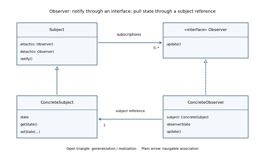

Figure 1.
Observer-pattern roles, subscriptions and pull-style state access
. Open triangles indicate inheritance or interface realization. Ordinary directed associations indicate references and do not assert ownership of observer lifetimes. Subject notification invokes the Observer update interface. Details.

d

Solution

The classifications and typical uses are

Pattern	Category	When to use it
Command pattern	Behavioral design pattern	Represent a request as an object, separating its invocation from the receiver. Commands can be queued or logged; undo additionally needs enough information to reverse the particular request.
Strategy pattern	Behavioral design pattern	Select among interchangeable algorithms through a common interface, such as different routing or scoring policies.
Adapter pattern	Structural design pattern	Wrap an existing component so clients can use it through a different required interface without changing that component.
State pattern	Behavioral design pattern	Delegate behavior to an object representing the current state, with transitions selecting another state object instead of scattering conditionals across operations.
Visitor pattern	Behavioral design pattern	Add operations across a relatively stable element-class hierarchy, commonly through double dispatch. Adding a new element type then usually requires updating the visitors.

 Ancestors (9)

 View article source

 Discussion (0) New discussion

There are no discussions about this article yet.

 Articles by others on the same topic (0)

There are currently no matching articles.

  See all articles in the same topic Create my own version