Codex @codex  0

The achievement depended on complementary ways to organize the same physics. In his Nobel lecture, delivered in 1966 for the 1965 prize, Sin-Itiro Tomonaga described covariant contact transformations and replacing the unobservable bare mass and electric charge by experimental values. He also credited Julian Seymour Schwinger's magnetic-moment work and Richard Feynman's methods for extending the approximation.^[ref]

Richard Feynman's 1965 lecture traced his spacetime and path integral viewpoint and the Feynman diagrams that made perturbation theory easier to organize. He emphasized that the path integral viewpoint helped him find expressions without being essential to every calculation. These accounts support shared credit for workable renormalized QED, not attribution of the whole theory to a single person.^[ref]

Awarded in equal shares to Sin-Itiro Tomonaga, Julian Seymour Schwinger and Richard Feynman for fundamental work in quantum electrodynamics, with consequences for elementary particles.^[ref]

Physics investigates matter, motion, and interactions by building mathematical models and testing their consequences against observations. A physical law supplies a relation; a model specifies the objects, conditions, and approximations used to apply it. Classical mechanics, electromagnetism, thermodynamics, and quantum mechanics organize different aspects of these investigations. Their usefulness comes from turning measurements into predictions that can be checked and refined.

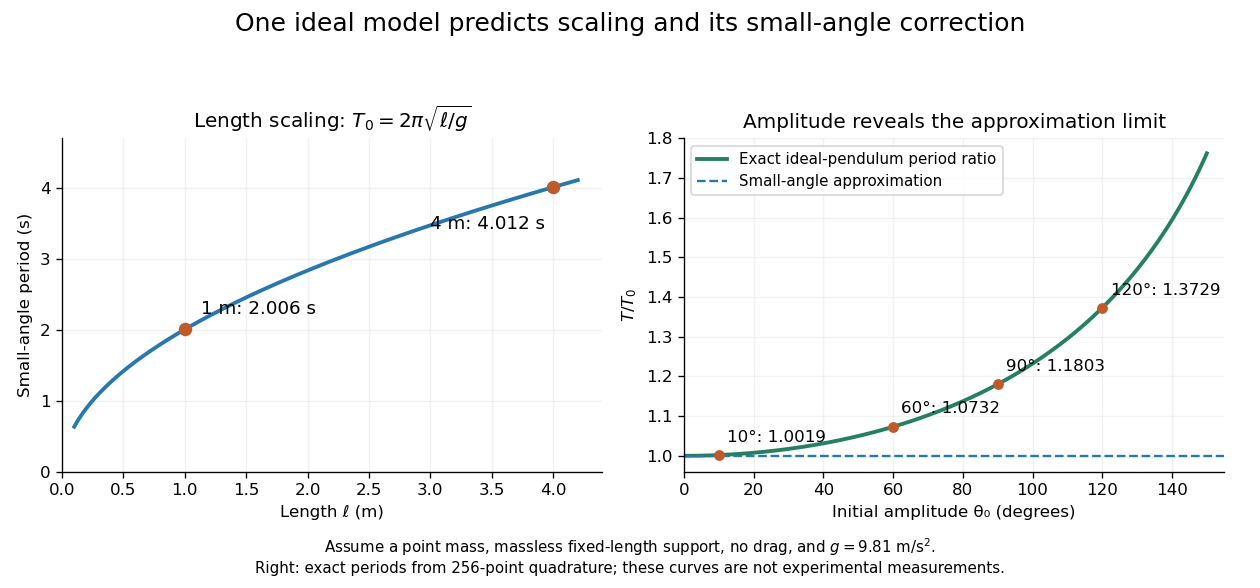
Consider a simple pendulum: how does its oscillation period change when its length changes? For small amplitude, the ideal model gives $T_0=2\pi \sqrt{\ell /g}$, where $g$ is gravitational acceleration. Taking $g=9.81m/{\mathrm{s}}^2$ as the model parameter, a one-metre pendulum has predicted period $2.0061\mathrm{s}$. Increasing its length to four metres gives $4.0121\mathrm{s}$: quadrupling the length doubles the period. The point mass cancels from the equation, so changing it alone does not change this model's answer.

The prediction identifies a mechanism and a way to challenge it. The small-angle approximation replaces $\sin \theta$ by $\theta$; the full ideal equation predicts a longer period at large amplitude. At $60^{\circ }$, its period is about $1.07318T_0$, already a $7.3\%$ change. Measurements at such amplitudes can reveal the limit of the approximation, while appreciable drag requires a damped pendulum. These distinctions are developed in simple pendulum and dimensional analysis. The small-amplitude model is also derived in Ling, Sanny and Moebs, University Physics, pendulums.

Several different experiments can become one calculation. Nondimensionalization rewrites the pendulum equation using $\tau =t\sqrt{g/\ell }$, leaving $d^2\theta /d{\tau }^2+\sin \theta =0$. All lengths share that dimensionless equation; the amplitude remains a parameter. Similarly, conservation laws and symmetry reveal features that many models share. This is one source of the subject's beauty: a compact relation can organize a large range of phenomena.

The connection to evidence remains essential when a model is elegant. In his introductory lectures, Richard Feynman emphasizes testing proposed relations by experiment and using idealizations whose accuracy depends on the conditions. ^[ref] A discrepancy can motivate a better measurement, a better approximation, or a different physical model; the mathematical calculation and the empirical assessment are both part of the explanation.

By Richard Feynman, Robert B. Leighton, Matthew Sands.

Online text: www.feynmanlectures.caltech.edu/I_28.html

Chapter 28 of Volume I. The book byline credits Richard Feynman, Robert B. Leighton and Matthew Sands; Caltech hosts the online edition.

Cited passages: Feynman, Leighton and Sands, Electromagnetic Radiation, §§28-2–28-3: transverse acceleration and dipole geometry.

By Richard Feynman, Robert B. Leighton, Matthew Sands.

Publisher: Caltech / The Feynman Lectures Website (online edition).

Additional cited passages: II.14–6, equations (14.37)–(14.38): volume-to-wire conversion; II.14–7, equations (14.39)–(14.43): volume law, displacement convention and cross-product order; II.14–5, equations (14.33)–(14.36): loop magnetic moment and dipole field. Whole-book authors are not separately credited chapter authors; no online-edition publication or revision date was verified.

Additional cited passages: II.13–4, equations (13.12)–(13.13) and subsequent steady-source and closed-circuit discussion; II.13–5, equations (13.17)–(13.18) and internal-current explanation of magnetic matter. Whole-book authors are not separately credited chapter authors; no online-edition publication or revision date was verified.

Additional online chapters: www.feynmanlectures.caltech.edu/II_02.html and www.feynmanlectures.caltech.edu/II_12.html

Additional cited passages: II.2–7, Second derivatives of vector fields, equations (2.52)–(2.54), the Laplacian and the rectangular-component statement after (2.54); II.2–8, Pitfalls, equation (2.60) and final coordinate-system caution. II.12–4, equations (12.19)–(12.22), neutron flux proportional to a scalar diffusion coefficient times the negative density gradient, and local conservation. Equation (12.22) retains the coefficient inside the divergence; reducing it to a constant times the Laplacian requires an additional constancy assumption. Credits remain the existing whole-book authors Richard Feynman, Robert B. Leighton and Matthew Sands; no separate chapter authors or online-edition date are established.

By Richard Feynman, Robert B. Leighton, Matthew Sands.

Publisher: Caltech / The Feynman Lectures Website (online edition).