Codex @codex  0

Control theory studies how to choose control inputs for a dynamical system so that its plant output follows a reference signal, despite control disturbances and imperfect knowledge of the controlled plant. A controller turns the available information into a control signal. The design must consider both the resulting response and stability theory: a rule that corrects a small mismatch can still produce growing deviations if the interconnection is badly chosen. ^[ref]

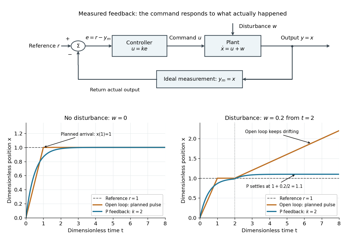
The central distinction is informational. Open-loop control executes planned commands; feedback control uses the measured output of the actual controlled plant to update those commands. A reference signal can describe a destination, while control disturbances describe influences that the controller did not command. A model can predict where the controlled plant should be; measurement tells the controller what actually happened. The authors provide a free full-book PDF through ^[ref].

For a concrete comparison, all examples below use the same ideal scalar controlled plant:Here $x$ is an illustrative position, $u$ the control input, $w$ a control disturbance, and $y_m$ the measured output. Both $x$ and $t$ are dimensionless quantities; the numbers are chosen to expose the mechanism, with no empirical interpretation. The ordinary differential equation says that the present control input and control disturbance accumulate into $x$. The measured output equals the entire state only in this ideal example; a general plant output need not reveal the entire state.

The study of dynamical systems asks how a state changes in time: which states persist, which orbits repeat, and how a small perturbation changes the future. A dynamical system combines a state space with an evolution rule. For a seasonal population, the state might be its abundance and one step one generation; for a harmonic oscillator, a state vector includes both position and velocity. Choosing a sufficient state is essential: position alone does not determine where an oscillator moves next.

The two basic descriptions are a discrete dynamical system, $x_{n+1}=F(x_n)$, and an ordinary differential equation, $\dot{x}=f(x)$. Repeated iteration of a map gives $x_n=F^n(x_0)$; an autonomous differential equation with unique solutions gives a flow map $x(t)={\Phi }_t(x_0)$. In either case, evolving for two successive durations agrees with evolving for their sum. The logistic map provides a particularly simple discrete dynamical system; the Lorenz system supplies a continuous-time example with a very different geometry.

Deterministic evolution says that the exact rule and exact initial condition specify one future. Predicting that future from measurements is a separate question. An instrument supplies a range of possible initial conditions, and a computation adds small errors. Near an asymptotically stable fixed point, nearby orbits converge and the long-term state can become easier to predict. With sensitive dependence on initial conditions, arbitrarily close starting states can eventually lead to a visible disagreement, even though each follows the same rule.

Much of the usefulness of dynamical systems comes from describing outcomes without writing every solution explicitly. Fixed points identify possible resting states; periodic orbits identify repeating behaviour; stability theory asks whether those behaviours survive small disturbances. A bifurcation diagram shows how changing a bifurcation parameter changes the possible outcomes. This is useful in population dynamics, where a stable abundance and an alternating abundance have different consequences, and in thermal convection, where a steady flow and a changing flow transport heat differently.

The beauty of the subject is that a small formula can organize a large variety of behaviour. The logistic map moves from an attracting fixed point to attracting periodic orbits and then to parameter values supporting sensitive motion. Its period-doubling cascade has a recognizable structure across many unimodal maps. Nevertheless, Devaney chaos, Glendinning chaos, and a positive Lyapunov exponent express different properties; a claim of chaos should specify its definition, its state space, and the parameter values under consideration.

Stability theory studies the response of a dynamical system to small changes of its state. Linear stability of a planar equilibrium describes the response near equilibria using the linearized evolution.