A dynamical system combines a state space with a rule for evolution in time. A discrete rule sends a complete state to , while a continuous model can specify . The state must include enough information for the chosen rule: a harmonic oscillator needs both position and velocity, because equal positions with opposite velocities have different immediate futures.
The same model can be studied through several questions. An equilibrium point stays fixed, a periodic orbit repeats, and a basin of attraction describes which initial states approach a selected long-term behavior. Changing a parameter can cause a bifurcation. These qualitative properties can be useful even when no explicit formula for every trajectory is available. Deterministic evolution also requires well-defined forward solutions; merely writing a differential equation does not establish existence or uniqueness of its initial value problem.
A dynamical observable is a function or that assigns a measurable quantity to each state of a dynamical system. If the dynamics is , the observed sequence from state is . The state space may be high dimensional even when this record is scalar.
For a harmonic oscillator with state , position is one dynamical observable; energy is another. Position generally oscillates, while energy is constant along an ideal conservative trajectory. Composition describes evolution of the measured quantity instead of evolution of states. Its time average, , is the object compared with a space integral in ergodic theory.
For a map and a given dynamical observable , the additive cohomological equation asks for a function satisfyingWhen such exists, is a difference accumulated between consecutive states. Summing along a trajectory makes the intermediate terms cancel:Thus bounded forces these sums to remain bounded, and any periodic orbit of period must have sum zero. These are necessary conditions, not a universal existence theorem.
For the circle rotation , try and . Then when the denominator is nonzero. If it vanishes, this mode is an obstruction; if it is very small, the coefficient is large. This explains how a simple equation leads to delicate regularity questions in dynamical systems.
A time average measures an dynamical observable along a single trajectory of a dynamical system. For a flow , define . If the limit as exists, it is the long-time average at initial state . For a discrete map , the corresponding expression is .
If , the average tends to zero although the observable never settles to a constant. The Birkhoff ergodic theorem supplies almost-everywhere existence for integrable observables under a probability-preserving map. Equality with a spatial average requires the appropriate ergodicity assumption; existence alone does not imply it.
An additive cocycle over a dynamical system records a quantity accumulated along a flow. It satisfies and : accumulation over two intervals equals accumulation over the first interval plus accumulation over the second interval from the evolved state.
For an dynamical observable , the integral is an example, as splitting the integral at proves the identity. A coboundary has the special form . Matrix-valued multiplicative versions replace addition by an ordered product; the order matters when the matrices do not commute.
Synchronization of oscillators occurs when interacting or driven oscillators acquire a sustained relation between their phases or frequencies. Equal amplitudes are not required. In one simple phase model, a relative phase obeys , where is the uncoupled frequency mismatch and the coupling strength.
When , a fixed relative phase exists; the branch with is stable because the linearized restoring coefficient is . The Kuramoto model extends this competition between mismatch and coupling to a population of phase oscillators.[ref]
From Kuramoto to Crawford: exploring the onset of synchronization in populations of coupled oscillators by Steven H. Strogatz. Sections 2–3, phase reduction and collective synchronization
A state variable is a coordinate used to describe the instantaneous condition of a dynamical system sufficiently completely to determine its future evolution under a specified model and input. For a simple pendulum, its angle and angular velocity form a state; angle alone generally does not, because the same position can be traversed in either direction.
A second-order ordinary differential equation becomes a first-order system by setting : and . The choice of state variables therefore reflects the memory required by the model, and differs from merely listing measured outputs.
Repulsion in a dynamical system describes nearby trajectories moving away from an invariant state or set in forward time. For a scalar discrete dynamical system, a fixed-point multiplier with modulus greater than one gives local repulsion.
A forward-invariant set is a subset of a state space that contains every future state of each trajectory starting in it. For a discrete dynamical system with update map , the condition isMathematical induction then gives for every nonnegative integer . For a flow map, the analogous condition is for every forward time for which the solution exists.
Forward invariance does not require equality or backward invariance. For , the interval is forward invariant because , but the inverse image of one is two, outside . By contrast, the singleton is invariant in both directions.
This is useful before an exact solution is available. A forward-invariant positive interval prevents a population model from generating negative states and supplies an upper bound for all later iterates. The positive invariant interval for a cubic biological population map derives such a region by direct inequalities. Being bounded in a forward-invariant set does not alone imply convergence to one equilibrium point.
An invariant interval for a scalar map is an interval whose points remain in that interval under every forward iterate. Here invariance means forward invariance and does not assert surjectivity onto the interval.
For the discrete dynamical system withevery positive starting value satisfying has positive later iterates. The useful invariant interval is .
First, for every ,because the quadratic has positive leading coefficient and discriminant . Thus a positive first image lies below .
Second, on the cubic product can be negative only for . On that interval its magnitude is at most , so throughout . Together the bounds give . Mathematical induction then keeps all later values in that positive bounded interval.
The hypothesis on the first image is necessary: a positive starting population outside the invariant region need not have a positive image. The interval argument supplies positivity and boundedness; it does not by itself classify the eventual orbit.
A semiconjugacy from to is an intertwining map :In a topological factor-map convention, is also continuous and onto. Authors using the term for an arbitrary intertwining map should state that weaker convention. If is a homeomorphism, the relation is a topological conjugacy.
The identity transports every forward orbit. Induction gives , so iterating in the larger space and then projecting agrees with projecting first and then iterating. The map can merge different states, so the projected dynamics need not retain all information about the original orbit.
For example, let on the circle, on , and . ThenThus the doubling map maps onto the parameter-four logistic map by a continuous semiconjugacy. Since , it is not one-to-one and does not give a topological conjugacy by this map.
The forward orbit of a state is the collection of states reached as time advances. For a discrete dynamical system ,For a flow map , the analogous set is over the times for which the solution exists. The initial state is included; its future accumulation points instead form the omega-limit set.
For example, with gives . Zero is approached but is not one of those iterates, so the forward orbit differs from its closure. Forward evolution also need not determine a unique past: sends both and to . The distinction matters when discussing attraction or invariance for a map that cannot be inverted.
The box-ball system is a discrete cellular automaton with a row of boxes, each either empty or holding one ball. Consider finitely many balls and unlimited empty boxes to the right. During one update, process the original balls from left to right and move each exactly once to the nearest currently empty box on its right. The ordering and the instruction to move each ball only once are part of the evolution rule.
An isolated block of three balls in boxes moves to in one update. More generally, an isolated block of balls moves boxes per step, preserving its shape. Interacting patterns have a soliton interpretation: localized structures re-emerge with conserved identities, and the system has further conserved quantities.[ref]
A Soliton Cellular Automaton by Daisuke Takahashi and Junkichi Satsuma. Publisher abstract: solitary-wave interactions preserve identities; infinitely many conserved quantities
This gives a particularly concrete setting in which a simple integer update rule produces organized wave-like motion.Evolution is deterministic when a specified initial condition and evolution rule select a unique future orbit. For a discrete dynamical system, applying the same map to the same state gives the same next state. For an ordinary differential equation, uniqueness of the initial value problem is required; merely writing a differential equation does not guarantee it.
Determinism permits both asymptotic stability and sensitive dependence on initial conditions. It does not by itself imply reliable prediction from approximate measurements, and sensitivity does not introduce a random choice into the evolution rule.
The Lorenz system is the three-variable autonomous differential equationIt arose as a low-dimensional model of thermal convection. Edward Norton Lorenz used its numerical solutions in 1963 to study nonperiodic motion and sensitivity to the initial condition, with consequences for long-range weather forecasting.[ref]
Deterministic Nonperiodic Flow by Edward Norton Lorenz. Journal of the Atmospheric Sciences 20 (1963), pages 130–141: convection model, numerical nonperiodic solutions and forecasting implications
The equilibrium points follow directly from the equations. For and , the first gives and the third gives . The second then becomes . Thus the origin always exists, while for there are two additional equilibriawith matching signs in the first two coordinates. The symmetry exchanges them.
The Equilibrium bifurcations of the Lorenz system determine how their stability changes. The separate instantaneous Lorenz error growth at a zero-y crossing calculation concerns a perturbation at one instant; it should not be confused with the long-term Lyapunov exponent.
For positive , the origin of the Lorenz system loses stability at and two equilibria emerge stably. Center-manifold projection gives , proving a supercritical pitchfork. The nonzero-branch characteristic polynomial is . If these equilibria remain stable for all . Otherwise their transverse Hopf crossing occurs at the displayed parameter, with frequency squared . Its cubic Hopf coefficient is positive, so this Hopf is subcritical, producing an unstable small periodic orbit on the stable-equilibrium side. A zero eigenvalue detects the pitchfork, while the Hopf condition uses the Routh-Hurwitz equality; neither alone determines nonlinear criticality without the corresponding normal-form calculation.
Consider the Lorenz system with and , at a state where . An infinitesimal error evolves by , where is the Jacobian matrix. Its squared Euclidean norm satisfiesAt that crossing, the skew couplings involving cancel, leavingThe planar block has negative trace and determinant . It has a positive eigenvalue exactly whenThus some error direction initially grows for either or . The vertical direction initially contracts.
For , , and , the eigenvalues of are . The most rapidly growing unit direction is , with instantaneous logarithmic norm growth . The factor of two distinguishes squared-norm growth from norm growth.
This is a local criterion at the specified state. Later rotation of the perturbation direction can change its growth, so it does not prove a positive asymptotic Lyapunov exponent.
The Feigenbaum period-doubling map is the universal, even, quadratic-critical fixed map associated with repeated period-doubling bifurcations. One normalization isComposing twice and rescaling therefore reproduces the same graph. This self-similarity is the mechanism behind a common spatial scaling in otherwise different one-dimensional maps with a quadratic maximum.[ref]
Quantitative Universality for a Class of Nonlinear Transformations by Mitchell Feigenbaum. 1978: universal spatial scaling and the period-doubling functional equation
The quadratic maximum means and . Twice applying the chain rule at zero givesThe term involving vanishes, and cancellation is legitimate because the maximum is nondegenerate. Thus the endpoint derivative is determined by the spatial scaling.
Writing makes the successive central intervals shrink by the factor . Their iterates generate the Feigenbaum attractor; nonuniform interval lengths are encoded by the Feigenbaum geometric potential. The constant here describes spatial scaling, rather than the spacing of successive bifurcation parameter values.
The Feigenbaum geometric potential is a bounded negative symbolic potential encoding the lengths of nested intervals of the Feigenbaum attractor. In an appropriate binary coding,and changing only the distant tail of an address changes by an exponentially small amount. For odd interval labels, a sum along reversed address prefixes satisfieswith a bound independent of the depth and address. Even-label intervals have lengths comparable to neighboring odd-label intervals. These uniform estimates connect geometric lengths with thermodynamic formalism.[ref]
Feigenbaum universality and the thermodynamic formalism by E. B. Vul and others. Thermodynamic description of the period-doubling geometry
[ref]Multifractality of the Feigenbaum attractor and fractional derivatives by Uriel Frisch and others. Section 2.1, equations (8)–(14): bounded potential, decaying variations and interval-length comparisons
The bounded logarithmic error is important. For fixed real , exponentiation givesAfter summing and taking , the error is at most , which vanishes. Thus geometric partition sums and symbolic partition sums give the same limiting topological pressure. The almost-additive partition-function limit supplies existence under the bounded-distortion hypotheses; bounded negative potentials give a strictly decreasing pressure.
This potential measures geometric contraction across partition levels. It is not an unbounded derivative potential evaluated at the critical point, where , and partition depth is distinct from elapsed orbit time.
Odd-address intervals lie in the first image of the central restrictive interval, away from the critical point. The derivative of the Feigenbaum map is bounded above and away from zero there, so the next even interval has comparable length by the mean value theorem. For the wraparound image, makes its length a fixed fraction of the central interval. Thus the odd and full partition length-power sums differ only by constant factors for each fixed real exponent, and have the same exponential growth rate.
For the normalized Feigenbaum map, put and defineThe Feigenbaum attractor is the nested intersection . Each level interval has two children, and the largest interval length tends to zero. Consequently every compatible infinite binary address selects one point of this Cantor set.[ref]
At level , the intervals are visited cyclically: the label changes from to modulo . Expressing in binary therefore turns iteration on into the dyadic adding machine. One adds one with carries, rather than discarding the first symbol as in a full shift. For example, addresses written with the least significant digit first begin .
There are geometric pieces at depth , but those pieces are visited in a cycle. Counting them does not make the time evolution a two-symbol full shift. The Feigenbaum geometric potential uses this depth to study spatial contraction and Hausdorff dimension.
The dyadic adding machine is addition by one on the space of infinite binary digit sequences, interpreted with the least significant digit first. Carries propagate toward later digits: . The all-ones sequence maps to the all-zeros sequence.
Equivalently, it is the compatible collection of cyclic maps for all , or translation by one on the 2-adic integers. Every orbit visits every finite binary cylinder and is therefore dense. At the Feigenbaum attractor, this describes the order of visits to nested intervals; it is not the digit-discarding evolution of a full shift.
A piecewise differentiable interval map is uniformly expanding when a constant bounds the derivative on every smooth branch:With a finite partition into monotone branches, a point's itinerary records which branch contains each iterate. A length- cylinder consists of points with the same first branch labels. Wherever this composition is smooth, the chain rule gives .
The mean value theorem then bounds the diameter of a cylinder by the length of the original interval times . Inverse branches therefore determine starting points with exponentially improving spatial precision as more itinerary symbols are specified.
For the doubling map on , the two branches have slope two and the level- cylinders are half-open intervals of length . Their labels are the first digits of the binary expansion. Endpoint conventions matter for unique coding, but not for the cylinder-length estimate.
Expansion describes the map's geometry. A symbolic potential separately specifies statistical weights, so expansion alone does not make every Gibbs measure absolutely continuous. The geometric potential of an expanding map uses the inverse derivative to select weights adapted to interval length.
For a differentiable uniformly expanding interval map, the geometric potential of an expanding map isThe exponential of its length- orbit sum is the reciprocal derivative magnitude . This weight is geometric: an inverse branch contracts interval lengths by that factor.
The corresponding Perron-Frobenius operator transports a density by summing contributions from inverse branches:For a finite smooth full-branch expanding map, standard bounded-distortion hypotheses give a positive regular fixed density , normalized by . The identity means that is an invariant measure. The cylinder averages of an invariant density explain how the geometric cylinder weights recover that density.
For the doubling map, there are two inverse branches andThe constant density is fixed, giving Lebesgue measure. Choosing an unequal-symbol potential instead produces a different Gibbs measure; an arbitrary Gibbs measure need not be absolutely continuous. Thus the potential, rather than the symbolic alphabet alone, determines whether the measure agrees with geometric length.
The Perron-Frobenius operator transports a density under a map. For a piecewise smooth expanding interval map , relative to Lebesgue measure,Each inverse branch contributes its incoming density times its length-contraction factor. A change of variables gives , proving that probability is transported correctly.
For the doubling map, . Thus the constant density is fixed. More generally, a normalized nonnegative fixed density determines an absolutely continuous invariant measure; a constant density need not be fixed for an arbitrary expanding map.
Let a uniformly expanding interval map have cylinders whose maximum length at level is at most , with . Suppose an invariant probability density is Lipschitz continuous with constant and satisfies . Its cylinder probabilities are . Define the piecewise constant logarithmic averageThe average of over differs from by at most . Since the logarithm has derivative at most on this range,Thus the cylinder data recover the logarithm of the density uniformly at a geometric rate.
Conversely, take consistent positive cylinder probabilities and suppose these converge uniformly to a finite function . Put . If , integrating over every level- cylinder compares its -mass with its assigned probability within factors . Subdivide any fixed cylinder into these finer cylinders and sum: consistency gives the same multiplicative bounds for the fixed cylinder. Letting proves .
Shrinking cylinders determine the Borel probability measure, so the geometric image of the symbolic law is exactly . Use a consistent convention at branch endpoints; bounded limiting cylinder densities imply zero mass at individual endpoints. If the symbolic law is shift invariant, the coding relation transfers that invariance to the interval map. This converse is much stronger than inspecting a density ratio along just one itinerary.
Thermodynamic formalism studies weighted trajectories through partition functions, topological pressure and invariant measures. A symbolic potential assigns an orbit segment the weight , where is its accumulated potential. Summing these weights gives ; the limiting logarithmic normalization per step is the pressure.
A one-symbol example shows the mechanism. On a two-symbol full shift, let and . ThenNormalizing gives independent symbol probabilities and . The associated Gibbs measure is therefore an orbit-weight law, not a uniform choice unless .
The same construction can encode geometry. A geometric potential of an expanding map records inverse-branch contraction, while the Feigenbaum geometric potential encodes lengths in a nested partition. Their pressure functions organize spatial scaling and dimension calculations. In that second example, the partition depth is a geometric scale index and should not automatically be identified with elapsed orbit time.
This explains both the usefulness and the limitation of the statistical-mechanics analogy: changing the potential changes which trajectories or geometric pieces receive weight. An arbitrary Gibbs measure need not be absolutely continuous, even when its underlying interval map is expanding.
A Gibbs measure gives probabilities controlled by exponential weights from a potential. The precise convention must be specified: finite-volume conditional distributions and symbolic orbit-weight bounds are related formulations with different hypotheses.
For a finite-alphabet full shift, a standard symbolic Gibbs condition for a probability measure is that a constant satisfyfor every length- word and every in its cylinder set . Here , and is topological pressure. The same constant must work for every word and every length. Summable variations make the orbit-weight comparison within one cylinder uniform. In applications to equilibrium states, shift invariance is also required.
For a one-symbol potential , where every and , the independent-symbol law hasThe bound is exact with . Equal symbol probabilities and unequal symbol probabilities are both Gibbs laws, although their geometric images can be very different: an arbitrary Gibbs measure need not be absolutely continuous.
An arbitrary unnormalized list of one-sided weights need not give consistent conditional probabilities for every finite horizon. Normalization and compatibility are part of constructing the measure, rather than consequences of calling the weights Gibbs.
A Gibbs measure is determined by its potential, rather than by geometric volume alone. The doubling map gives a concrete counterexample. Away from dyadic rationals, write . Give the binary digits independent probabilities and , with .
A length- cylinder set with ones then has probability . This is the Gibbs measure for the one-symbol potential when and otherwise. The normalized topological pressure is zero because the length- weights sum to .
Let be the set of numbers whose binary expansion has limiting frequency of the digit one. The strong law of large numbers gives . Under Lebesgue measure, binary digits are independent fair digits: every length- cylinder has length . The same strong law of large numbers therefore gives digit frequency almost surely. For , it follows that .
Thus and Lebesgue measure are mutually singular measures. The ambiguity of dyadic expansions affects only a countable set with zero mass under both measures. The geometric choice is precisely , when cylinder probabilities equal cylinder lengths.
Comparing ratios on a few cylinders would be a weaker argument. Failure of uniform convergence to a positive bounded density does not exclude every possible integrable density; the full-measure set proves actual singularity.
For a finite full shift with alphabet and a continuous potential of summable variations, topological pressure is the limiting logarithmic weight per step:Here concatenates a finite word and a fixed reference tail, and is the left shift. Summable variations bound the effect of changing that tail by a constant independent of . The almost-additive partition-function limit consequently proves existence and tail independence.
For a fixed potential , the function is convex. At finite , differentiating twice gives the variance of the orbit sum under its normalized weights, divided by , which is nonnegative. Passing to the limit preserves convexity.
If , then for each orbit weight is multiplied by a factor between and . HencePressure is therefore strictly decreasing and Lipschitz continuous. If the alphabet has symbols, and as . The intermediate value theorem then gives exactly one positive zero. For a one-symbol alphabet the zero is instead at ; the alphabet-size qualification is essential.
For example, the constant potential , with , has and . Its zero is , making the role of alphabet size explicit.
The sequences and are respectively subadditive and superadditive. Apply Fekete's lemma to the first and its negative to the second; their normalized difference is , so their limits coincide. For full-shift weighted orbit sums, summable variations of the potential bound the energy change at a concatenation boundary, giving this estimate for the logarithm of the partition function. A fixed initial symbol or fixed remote tail changes only a bounded normalization and not the limit.
A symbolic potential is a real-valued function on a symbolic sequence space, for example on a finite full shift. Its orbit sumweights a length- orbit segment in a partition function. Here is the left shift. The potential can encode geometric contraction or a chosen statistical preference; it is not determined by the alphabet alone.
Its variation at depth isSummable variations mean . If and agree on their first symbols, their shifted sequences agree for symbols at step . ThereforeThe right side stays bounded independently of . This uniform orbit-weight distortion is what allows a reference tail to be changed without changing topological pressure.
For a potential depending only on , every variation with is zero. The choice generates independent-symbol weights, while a geometric potential of an expanding map instead describes inverse-branch contraction.
An integer matrix with determinant defines a toral automorphismon the real torus . Integer entries make the map independent of the chosen representative. The inverse matrix also has integer entries, so the transformation is invertible. It preserves normalized Haar measure.
The map is a mixing measure-preserving transformation exactly when no eigenvalue of is a root of unity. This can be proved with characters of a real torus , since . Orthogonality givesIf no eigenvalue is a root of unity, a nonzero integer frequency cannot repeat: a repetition would give for some . It therefore eventually leaves every finite set of frequencies. The displayed correlations prove mixing first for trigonometric polynomials, then for square-integrable functions by approximation.
Conversely, a root-of-unity eigenvalue makes singular for some . As an integer matrix it has a nonzero rational kernel vector, which can be scaled to a nonzero integer vector . The nonconstant character is then invariant under , obstructing mixing. The cat map is a mixing example, while the identity matrix gives an invertible measure-preserving map that is not mixing.
The imperfect soft Duffing-van der Pol oscillatorcombines a softening restoring force, velocity-dependent damping and the symmetry-breaking term . The equilibrium points are and , whenever the latter are real. The associated Jacobian matrix has trace and determinant .
At , the equilibrium equation has the reflection symmetry . For , the branch near zero crosses the zero branch at , giving the generic transcritical bifurcation when . The two nonzero roots meet at , , giving a generic saddle-node bifurcation when . The excluded trace-zero cases have an additional linear degeneracy and require further analysis.
The mechanical energyhas the exact derivative . Thus the sign of energy input can change with displacement even at a fixed value of .
For , the two outer equilibria are saddle equilibria. Their potential barriers are generally unequal when , so a symmetric saddle connection can split into distinct directed connections under an imperfection. The weak-damping heteroclinic splitting of a tilted quartic oscillator calculates their leading parameter curves. Local equilibrium formulas alone do not guarantee a limit cycle or determine its global termination.
Pattern formation is the development of spatial structure in a system. A common mechanism is the loss of stability of a uniform state to disturbances at a preferred nonzero wavenumber. In Rayleigh-Bénard convection, heating a fluid layer from below can destabilize the conducting state and produce organized convection rolls. In a reaction-diffusion equation, reaction and transport can instead select a spatial concentration pattern.
A linear calculation separates the possible scales. Write a small disturbance as a Fourier mode . Positive real part of means that mode initially grows, and the fastest growing wavenumbers often set the first visible scale. The Swift–Hohenberg equation has , so at small positive it amplifies a band near .
Linear growth is only the onset calculation. A growing disturbance eventually becomes large enough for nonlinear terms to matter. Coupled amplitude equations can then describe competition between modes: one mode can suppress another, several can coexist, or the state can drift or oscillate. The resulting planform includes both the selected wavevectors and their relative amplitudes and phases.
A slowly varying phase modulation describes changes in a pattern's local position and orientation without immediately destroying its periodic structure. Its stability can differ from the stability of a uniform amplitude, as illustrated by the zigzag instability of parallel rolls.
A planform is the spatial arrangement of a pattern, especially its horizontal structure in a fluid layer. In a Fourier mode description it includes the active wavevectors, their relative amplitudes and their phases. Those data determine more than a list of preferred wavelengths.
For example, describes parallel bands, with wavevectors . Adding an equal perpendicular pair gives , a square-symmetric planform. Unequal coefficients retain the two directions but generally lose the symmetry exchanging them.
A common translation symmetry changes the phases by without changing the physical shape. Relative phase combinations that cannot be removed by a translation can distinguish different arrangements, as the translation invariants of Fourier-mode phases show. Thus choosing a planform identifies a symmetry type; the amplitude equations still have to determine whether that state exists and is stable.
A phase modulation changes the local position of a periodic pattern. If has period in its argument, a transverse modulation can be writtenA constant translates the entire pattern; a varying bends its constant-phase lines. For the basic profile , the local wavevector is . The orientation changes at first order in the slope, while the local wavenumber is .
In the method of multiple scales, a correction depends both on its fast coordinate and on its slow coordinate . Differentiating at fixed physical therefore uses the chain ruleFor instance, differentiates to , not just the second term. The translation-covariant phase expansion calculates the second derivative needed in solvability conditions. Omitting the fast-coordinate dependence can change the nonlinear coefficient of the reduced amplitude equation while leaving its linear coefficients unchanged.
Let , and . Two applications of the chain rule give . In a Fredholm solvability condition, the fourth term generally contributes to the coefficient of . It cannot be omitted merely because the fast-coordinate correction functions have been denoted by .
A zigzag instability is a long-wave transverse phase modulation of parallel rolls. In the modela small Fourier mode has growth rate . Thus the straight pattern is linearly stable for and unstable to sufficiently long transverse waves for .
When , the unstable band is . Differentiating with respect to gives the fastest growing scale and maximum growth . The fourth derivative stabilizes short waves rather than allowing arbitrarily fine structure to grow fastest.
Writing the slope as givesa conserved Cahn--Hilliard equation for the local orientation. When and , its homogeneous bulk potential has two minima at . These are preferred local slopes; boundary conditions and the conserved mean slope still constrain the complete pattern.
At a transverse phase-diffusion threshold the coefficient of the second spatial derivative is of order . Its product with two long-wave derivatives therefore has order , the same order as the stabilizing fourth derivative. This balance determines the slow time and retains both terms in the leading phase modulation equation.
The Swift–Hohenberg equation is a partial differential equation for pattern formation. In one spatial dimension, a cubic-quintic version isLinearizing at and substituting a Fourier mode gives . The first unstable modes therefore have wavenumber near one when becomes positive. Replacing one by inside the differential operator selects wavenumbers near .
There is also a useful Lyapunov functional. On a periodic interval, or with sufficient decay at infinity, defineTwice using integration by parts gives the functional derivative . The equation is therefore a gradient flow, andThis dissipative structure constrains the evolution without requiring the final spatial pattern to be uniform. For , the cubic term enhances finite amplitudes while the quintic term limits growth. Near onset, a slowly varying envelope can satisfy a quintic real Ginzburg-Landau equation.
In the mildly subcritical Swift–Hohenberg equation, set , and . The nonlinear and growth terms first balance at order , so . Quadratic detuning of the critical Fourier growth rate gives . At order , projection onto the kernel of the self-adjoint fast operator requires the resonant forcing to vanish. The cubic and quintic resonances have coefficients and , while the operator expansion gives . Thus .
A reflection-symmetric planar cubic model can be expressed in polar variables , , as and . A nonzero equilibrium therefore has , . Adding their squares gives . Each positive root determines an antipodal equilibrium pair. The determinant of the polar linearization there is and its trace is . These formulas distinguish folds of nonzero equilibria from symmetry-forced bifurcations at .
A Lyapunov exponent is the asymptotic exponential growth rate of an infinitesimal tangent displacement along a dynamical system. For a differentiable flow map, a starting point and a nonzero tangent vector , one convention iswhen the limit exists. A discrete dynamical system uses the derivative of the th iterate and divides by instead. The rate can depend on the point and the direction.
For the linear ordinary differential equation , an eigenvector with real eigenvalue evolves as , so its exponent is . Nonreal eigenvalues contribute their real parts to the growth rate. A polynomial factor from a Jordan block does not change the exponent because .
In a smooth velocity field, the tangent displacement obeys . Its instantaneous stretching rate depends on both the current Jacobian matrix and the current direction. Those can change along the trajectory, so averaging instantaneous largest eigenvalues need not give the actual largest Lyapunov exponent.
The infinitesimal qualification matters. Two trajectories at a fixed finite separation cannot grow apart exponentially forever inside a bounded region: their distance is bounded by the region's diameter. A positive tangent exponent instead concerns the derivative obtained by sending the initial perturbation to zero first. Finite errors follow the linear prediction only until they become large enough that nonlinear effects matter. Likewise, growth rates of moments of a random separation need not equal the exponent along a typical trajectory.
For a unit perturbation direction and Jacobian matrix , the instantaneous logarithmic growth rate of its Euclidean norm is , where . Indeed for . The eigenvalues of the symmetric matrix give the principal rates and its orthonormal eigenvectors give the principal directions. These directions generally rotate as the trajectory evolves; their instantaneous rates need not equal asymptotic Lyapunov exponents.
Multistability is coexistence of several stable long-term behaviors at the same fixed parameter values. Those behaviors can be equilibrium points, periodic orbits or more complicated attractors. Different basins of attraction select which behavior a trajectory reaches from its initial state.
For example, has attracting equilibria at and a repelling equilibrium at zero. A sufficiently large perturbation can move a state from one basin to the other, leaving a persistent change after the perturbation ends. This gives a simple mechanism for dynamical memory without changing the governing parameters. Bistability is the two-state case. Hysteresis additionally describes history-dependent switching under a changed control parameter; coexistence alone does not specify a complete hysteresis loop or its switching thresholds.
Coexistence of two stable long-time states at fixed parameters. Initial conditions and sufficiently strong perturbations can select different basins of attraction, allowing a dynamical system to retain a state-dependent memory.
A biochemical regulatory module with two stable states over a specified range of conditions. History-dependent thresholds distinguish hysteresis from a single steep response.
For an equilibrium point , a homoclinic orbit is a nonconstant trajectory withAt a hyperbolic equilibrium point, the trajectory leaves a neighborhood of along its unstable manifold and returns along its stable manifold. It never reaches in finite time when local solution uniqueness holds. Its closure includes the equilibrium and can form a loop-shaped separatrix.
A completely explicit example iswith Hamiltonian function . Its derivative is zero along every trajectory, and the origin is a saddle point with eigenvalues . The curvelies on . Differentiating gives and , while the hyperbolic secant tends to zero at both time infinities. Thus it is a homoclinic orbit. Changing both signs gives the second loop.
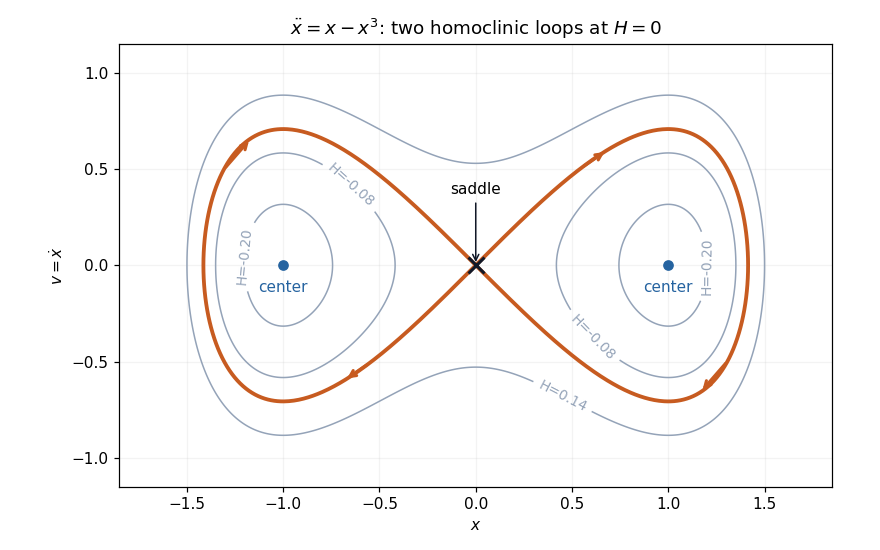
Two exact homoclinic orbits of the double-well oscillator return to the same saddle at infinite time
. Details. Each loop bounds periodic orbits around one potential minimum. This is an integrable Hamiltonian system, so a homoclinic loop by itself does not establish chaos. A Shilnikov bifurcation and a simple-zero Melnikov energy-balance method calculation require additional dimensional, spectral or forcing hypotheses.
For a hyperbolic equilibrium point with one unstable eigenvalue and weakest stable decay rate , the saddle index is . For a stable complex pair, use its real part. An incoming distance from the stable manifold takes time to reach an outgoing section at unstable coordinate magnitude . A stable coordinate is multiplied by , giving a power-law local passage. A smooth nondegenerate reinjection consequently has derivative tending to zero when and an unbounded leading derivative when . This determines local contraction or expansion near a homoclinic orbit; existence of a particular attractor also depends on the global return geometry.
At a planar saddle equilibrium with , positive saddle quantity is equivalent to saddle index . The local passage followed by the regular return has leading transverse map , . Its derivative diverges as , so a nearby periodic orbit created by the saddle-loop splitting is repelling. This local mechanism agrees with the growth of the unstable periodic orbit born at a subcritical Hopf bifurcation in the quadratic Bogdanov–Takens unfolding.
Near two homoclinic orbits of a planar saddle equilibrium with contracting ratio , the signed Poincaré return map has separate offsets . Two single-lobe periodic orbits exist for and , respectively. A two-lobe periodic orbit is represented by positive solving the displayed equations. Its boundary consists of the compound homoclinic orbit curves for and for , with . In a sufficiently small return domain the derivatives tend to zero, so each admissible symbolic branch has at most one attracting periodic orbit. Restricting to , gives the usual symmetric homoclinic gluing bifurcation.
A symmetric homoclinic gluing bifurcation joins two symmetry-related periodic orbits into one orbit that traverses both lobes of a figure-eight separatrix. At the transition, the two loops are homoclinic orbits to the same saddle equilibrium. The two original cycles spend increasingly long near that saddle before the connection is reached.
A signed transverse coordinate distinguishes the lobes. Reflection can make the corresponding return map odd, so fixed points and represent the separate cycles, while a two-cycle passing between positive and negative coordinates can represent the glued orbit. The signed gluing-map reduction describes the local power-law passage and the global reinjection; its coefficients and saddle eigenvalue ratio determine the existence and stability of these branches.
The geometry alone does not guarantee attracting cycles. For example, the exact Hamiltonian double-well homoclinic orbits form a figure-eight but are surrounded by conserved-energy families, rather than isolated attracting cycles. Dissipation, a suitable parameter unfolding and the return-map conditions must supply the gluing scenario. A damped double-well model with symmetry-related Hopf cycles is one setting in which those conditions can be investigated.
For a symmetric real saddle with one unstable direction and a strongly contracting transverse direction, composing the power-law local passage with a smooth global return gives this leading Poincaré return map, with and saddle index . It is undefined at the stable-manifold crossing . For , small fixed points on each branch are attracting for ; for an attracting alternating-sign period-two orbit satisfies , giving gluing of two one-lobe flow cycles into one two-lobe cycle. For and small , on , , the inverse branchesmap into and contract. Infinite branch choices define an invariant Cantor set with full two-symbol dynamics. In the two-dimensional return, transverse contraction turns this mechanism into a Smale horseshoe. An attracting Lorenz set additionally requires appropriate trapping and global-return properties.
Consider the branch return mapwith , , and nonzero return coordinates. After one iterate, . On these two sign sheets, define . Then and , givingThis scalar equation describes the signed gluing-map reduction.
A negative scalar fixed point has , so and the next is unchanged. The two sign choices therefore lift it to two symmetry-related fixed points of the original return map. A positive scalar fixed point instead has ; both and change sign on each step, giving one period-two orbit.
The value zero needs separate interpretation. In the underlying homoclinic orbit model it is the separatrix limit, where the flow's return time diverges. A formal continuous extension of the scalar formula at zero does not supply an ordinary finite-period periodic orbit. All branch iterations used to model finite flow returns must remain in the valid nonzero local domain.
For , a nonzero fixed point satisfiesAssume , and . A saddle-node bifurcation has multiplier , so it occurs at withAt either nonzero point, is nonzero and the parameter enters additively, giving the ordinary nondegenerate fold conditions.
When , define . The scalar extension has three fixed-point branches for : two stable outer branches and an unstable inner branch. For nonzero fixed points, their derivatives are below and above one because decreases with . At , the inner branch lies at the singular separatrix value; the signed gluing-map reduction explains why it is excluded as a finite-time flow return.
For fixed and from below, the fold magnitude has asymptotic value . This is the half-width; the total parameter interval has width . The exponentially narrow gluing-map cusp gives the exact rescaling. For approaching one, the formal fold coordinate instead tends to infinity, outside the local return-map region.
Fix in the signed gluing-map reduction and write with . The saddle-node curves of a signed power gluing map occur at parameter values , whereThus is the half-width of the three-branch interval, and is its total width.
To see the scale, use and . ThenSince and , the width decays faster than every positive power of . A parameter scan with an algebraic step size can therefore miss the coexistence interval entirely.
This is an essential exponential scaling, rather than the power-law fold separation in the ordinary smooth cubic cusp. The three branches counted here are scalar return-map branches. Their physical lifts differ: a negative scalar fixed point represents two symmetry-related cycles, while a positive one represents one cycle visiting both lobes. The singular zero value is a separatrix limit with infinite return time.
A Shilnikov bifurcation involves a homoclinic orbit to a saddle-focus equilibrium in three dimensions. Write its eigenvalues asand put . The Shilnikov return map combines contraction toward the equilibrium with arbitrarily many rotations before departure.
The sign of the saddle value separates two regimes. At a nondegenerate homoclinic connection with , the Shilnikov theorem gives countably many nearby saddle periodic orbits. When , the usual generic unfolding instead creates a locally attracting periodic orbit on the appropriate side. The boundary requires additional terms.[ref]
Shilnikov Bifurcation by Leonid Pavlovich Shilnikov and Andrey Shilnikov. Saddle quantity, the Shilnikov theorem and the contracting saddle-focus case
The spectral and nondegeneracy assumptions matter: a planar saddle loop has no rotating stable plane and does not supply this mechanism. The result is associated with Leonid Pavlovich Shilnikov; Andrey Shilnikov coauthored the cited account.
Near a saddle-focus equilibrium, linearized coordinates satisfy , and . A trajectory entering at a small positive coordinate takesto reach a fixed outgoing section. Hence with , while the accumulated angle is logarithmic in . Composing this passage with a smooth global return gives the leading scalar formwhere and the phase convention absorbs constant angular shifts. The map applies only on branches whose trajectories return to the section.[ref]
Shilnikov Bifurcation by Leonid Pavlovich Shilnikov and Andrey Shilnikov. Local saddle-focus passage and the oscillatory Poincaré return map
Differentiation givesFor , the envelope becomes unbounded as , but the derivative also has infinitely many zeros. The map therefore has strongly expanding branches, rather than uniform expansion everywhere.
The full two-dimensional return has Jacobian determinant of order in regular section coordinates: radial scaling contributes and conversion of polar coordinates contributes . For this contracts area near the singular limit, but area contraction alone does not prove that a scalar reduction is valid. A one-passage periodic trajectory has period , explaining the logarithmically diverging time near the homoclinic connection.
At a saddle-focus homoclinic orbit, the leading Shilnikov return map is , , with . If , its fixed points solve . Infinitely many solutions accumulate at zero near the zeros of the cosine, with successive size ratios tending to . The derivative is , so their expanding multiplier is unbounded. Narrow monotone strips near successive oscillations map across a common interval; inverse branches contract, supplying arbitrarily long symbolic itineraries and infinitely many saddle periodic orbits. Varying the splitting parameter shifts the graph vertically, producing accumulating fold and period-doubling thresholds and stable windows. The condition makes the local flow volume-contracting, whereas makes its saddle value positive.
ConsiderThe circle is a periodic orbit. Writing gives , while on the circle. Its normal Floquet multiplier is therefore .
Inside the circle, use the increasing angle as independent variable and set . Direct differentiation gives the linear ordinary differential equationLet . The solution with isAt the endpoint, and , so immediately before . A crossing of has slope . Thus there is no crossing on compatible with this terminal behavior. AlsoEvery crossing on has positive slope, giving a unique where . Hence for and tends to zero at both ends. At the incoming endpoint , so has a divergent integral. At the outgoing endpoint the zero is simple and the time integral diverges logarithmically. The curve is a homoclinic orbit to the origin.
Uniqueness for the angular scalar equation prevents positive-radius trajectories from crossing this loop. Inside it they approach the origin; outside it they approach the attracting circle. The origin therefore attracts an open set, but is not Lyapunov stable: points arbitrarily close to its outgoing branch follow trajectories to a fixed positive radius before returning or escaping. Attraction and stability are distinct properties.
An Anosov diffeomorphism is a continuously differentiable diffeomorphism of a compact smooth manifold with an invariant splitting of its tangent bundle into stable and unstable vector subbundles satisfying the displayed uniform exponential estimates for , with . Hyperbolic toral automorphisms give examples. An Anosov flow has a further one-dimensional invariant bundle along the flow direction; its definition is a distinct continuous-time version of uniform hyperbolicity.
A hyperbolic toral automorphism is a toral automorphism whose matrix has no eigenvalue on the unit circle. Here , so its determinant is . Invertibility merely over the real numbers would not suffice: multiplication by two on a circle is a many-to-one endomorphism, not an automorphism.
The real stable and unstable subspaces come from the generalized eigenspaces with eigenvalue modulus less than and greater than one. They give the same splitting at every point of the real torus. A Jordan block can add a polynomial factor to the powers of its eigenvalue; choosing a slightly weaker exponential rate absorbs that factor into a constant. Thus contraction forward on the stable subspace and backward on the unstable subspace is uniform over the whole torus, proving that the map is an Anosov diffeomorphism.
For the cat map, has eigenvalues . One is inside and the other outside the unit circle, and their product is one. The toral automorphism mixing criterion applies as well, since a root of unity would lie on that circle.
The cat map is the area-preserving map of the real torus given byIts integer matrix has determinant one and inverse , so reducing coordinates modulo one retains an invertible transformation of the torus.
Geometrically, stretches a unit square into a parallelogram. Cutting that parallelogram along the integer grid and translating its pieces by integer vectors brings it back into a unit square. Edges are identified on the torus, which is why cutting the drawing does not make the torus map discontinuous.
The eigenvalues and give one expanding and one contracting eigenvector. Their product one agrees with area preservation, while the absence of eigenvalues on the unit circle makes this a hyperbolic toral automorphism. The Fibonacci powers of the cat-map matrix give its iterates explicitly. Thus an integer matrix that is easy to multiply provides a concrete model of simultaneous uniform stretching, contraction and global wrapping.
Use the standard Fibonacci number convention , , . For the cat map matrix,At , the right side is . To prove the induction step, multiply it by . The top-left entry becomes , the top-right becomes , and the lower row follows from the same recurrence. This advances all indices by two.
For example, , so two iterations send to modulo one. The formula turns repeated matrix multiplication into an explicit integer recurrence; the exponential growth of the Fibonacci numbers agrees with the expanding eigenvalue of the cat map.
A smooth flow on a smooth manifold is a smooth map withThe identity implies , so each time map is a diffeomorphism. Its generating vector field is ; trajectories solve the autonomous differential equation .
For example, is a smooth flow on the real line, while is a rotation flow on a circle. The second has periodic trajectories, even though the same additive time parameter acts in both examples.
A smooth vector field initially gives only a local flow. The equation has , which blows up at for . On a closed manifold, compactness prevents escape in finite time and local existence can be continued for every real time. Thus every smooth vector field there generates a global smooth flow. On a noncompact manifold, global existence is a separate property.
An observable is a flow coboundary if it is the derivative of a function along a flow map. An integrated formulation isWhen is differentiable along the flow, this is , where is the generating vector field. Spatial regularity must be specified separately: may be smooth or merely Hölder continuous while still being differentiable along every flow line.
The function is a cocycle over a dynamical system. Its identity follows by adding the two differences from to and from to . Being a coboundary says that the accumulated observable can be recovered from endpoint values.
For a periodic orbit of period , the endpoint values coincide, so its integral of is zero. This is the periodic orbit obstruction. If is bounded, then the time average of also vanishes:For a transitive Anosov flow, the Livšic theorem identifies when the periodic-orbit obstruction is sufficient. This is stronger than checking just one average or finitely many periodic trajectories.
A periodic orbit obstruction is a necessary compatibility condition for solving a cohomological equation. If an dynamical observable is a flow coboundary, , where differentiates along the flow, then on a periodic orbit of period ,A nonzero integral therefore rules out a single-valued transfer function . Under suitable transitive Anosov flow and Hölder regularity hypotheses, the Livšic theorem provides a converse. Without those dynamical and regularity assumptions, vanishing periodic integrals alone is not a general existence theorem.[ref]
Abelian Livšic theorems for Anosov flows by Richard Sharp. Introduction, classical periodic-orbit theorem and equation (1.1)
For a volume form , define divergence by . The product rule for the Lie derivative gives . Consequently the flow preserves a smooth positive volume precisely when its divergence in any reference volume is a smooth flow coboundary. The displayed density has the minus sign dictated by this product rule.
A suspension flow turns a discrete-time map into continuous motion by moving along an extra time coordinate. For a diffeomorphism and constant roof one, form the mapping torusThe flow moves vertically at unit speed; each crossing of the top applies and re-enters at height zero. If has dimension , the suspension has dimension .
Suspending a hyperbolic toral automorphism gives an Anosov flow. After roof crossings, its transverse derivative is , so the base map's stable and unstable exponential bounds become the transverse flow bounds. A remaining fractional crossing has a uniformly bounded effect on a compact mapping torus. The vertical direction supplies the neutral flow direction. In particular, the two-dimensional cat map gives a three-dimensional suspension.
A constant roof also shows why this flow need not be mixing. The well-defined height function obeys . Under the product invariant probability measure its mean is zero, but its autocorrelation has modulus one for all . Thus even a mixing base map can produce a suspension with persistent clock correlations.
Write and . For an Anosov stable bundle, the new stable directions are , where . Exponential contraction makes this integral uniformly convergent. Differentiating the clock equation shows that its flow-direction coefficient after time is , which decays exponentially and has the same graph form at the new point. Negative-time integrals give the unstable graph. Compactness and positivity of compare old and new times uniformly, preserving the Anosov flow property.
An Anosov flow is a nonsingular smooth flow on a compact smooth manifold with a continuous derivative-invariant splittingHere is the generating vector field, the flow direction is one-dimensional, and in the usual nontrivial convention both and have positive dimension. Constants must work uniformly over all points, all and the corresponding tangent vectors:The stable bundle of an Anosov flow contracts forward; the unstable bundle of an Anosov flow contracts backward. The neutral direction along is essential: changing the starting point slightly along an orbit mainly shifts its clock, so that direction cannot be included in either uniform contraction estimate.
A suspension flow of the cat map gives a three-dimensional example. A positive time change of a smooth flow preserves the Anosov property on a compact manifold, although its stable and unstable bundles can tilt along the flow direction. These are uniform structural conditions, stronger than a sign observed in one finite-time Lyapunov exponent calculation.
The Anosov closing lemma turns a sufficiently close return of an Anosov flow into a nearby periodic orbit. On a compact manifold, uniform hyperbolicity ensures that an orbit segment returning close to its starting point is shadowed by a genuine closed orbit, with a small adjustment of the period and of the time parametrization.
Stable directions contract toward the shadowing orbit, while unstable directions are matched by choosing the appropriate nearby initial point. This makes periodic trajectories a tool for studying nonperiodic recurrence, for example when proving that periodic-orbit data control a cohomological equation. The time adjustment distinguishes the flow statement from its discrete-map counterpart.[ref]
Let a nonsingular smooth flow on a closed manifold be generated by . Suppose a continuous nondegenerate indefinite quadratic form on the transverse vector bundle has constant signature, is differentiable along the linearized flow, and has continuous positive-definite derivative there. Then the flow is an Anosov flow.[ref]
Here differentiating the form means differentiating . Compactness gives constants such that and . On the positive cone,so the form increases at least exponentially. Negative cones supply the analogous backward-time estimate. Strict cone invariance produces uniformly expanding and contracting transverse bundles; the full splitting also contains the neutral flow direction.
For a geodesic flow on a compact negatively curved surface, a transverse Jacobi field has scalar coordinates satisfying and , with Gaussian curvature . The indefinite form obeysfor every nonzero transverse vector. This directly verifies the criterion. The quotient by is essential: gives the neutral direction that cannot satisfy this strict transverse positivity. The estimates concern the form; constructing the invariant bundles is the additional cone argument, rather than an assertion that every positive-cone vector has monotonically growing norm.
Invariance gives for a stable direction. Boundedness of and exponential contraction make this zero; negative time does the same for unstable directions. Also . The Anosov splitting spans the tangent bundle, so and the function is constant on each connected component. This proof does not need an ergodicity hypothesis.
The Livšic theorem turns periodic-orbit data into a global derivative along a hyperbolic flow. Let be a transitive Anosov flow on a compact smooth manifold, with generating vector field , and let be a real Hölder continuous observable. There is a Hölder continuous function , differentiable along flow lines, satisfyingif and only if for every periodic orbit of period . The solution preserves the Hölder exponent.[ref]
Abelian Livšic theorems for Anosov flows by Richard Sharp. Introduction, equation (1.1) and its following paragraph: the classical all-periodic-orbit theorem
Necessity is immediate by putting in the identity. Two solutions differ by a continuous invariant function. Transitivity supplies a dense orbit; their difference is constant on that orbit, and continuity makes it constant everywhere. Thus the solution is unique up to an additive constant.
The harder sufficiency argument defines by integrating along a dense orbit. The Anosov closing lemma converts a sufficiently close return into a nearby periodic trajectory. Its vanishing integral and exponential shadowing bound the discrepancy between the endpoint values in terms of their distance. This gives Hölder control on the dense orbit and permits extension to the whole manifold.
When both the flow and are smooth, a separate regularity theorem gives smooth . This does not follow merely from the preceding continuity argument.[ref]
Canonical perturbation theory of Anosov systems, and regularity results for the Livsic cohomology equation by Rafael de la Llave and others (1985). Printed p. 92, Theorem 1 and proof sketch; p. 93 explicitly states the flow analogue
The theorem is named for A. N. Livšic.The unstable bundle consists of transverse directions exponentially contracted in negative time. Together with the stable bundle and the flow direction it gives the invariant splitting of an Anosov flow. Under a positive time change its graph coefficient is obtained from the convergent past integral .
The stable bundle consists of the transverse directions exponentially contracted in positive time. The unstable bundle has the corresponding negative-time property. A positive time change of a smooth flow can tilt these bundles in the flow direction, even though it preserves the underlying orbits.
The weak stable bundle adjoins the flow direction to the strong stable bundle. It is tangent to the weak stable foliation. For a geodesic flow on a hyperbolic surface, the canonical frame gives .
A nearly Hamiltonian system is a weak perturbation of a Hamiltonian system, writtenSince is skew-symmetric, its energy changes by . This identity is exact; it does not require replacing the perturbed trajectory by an unperturbed one.
For a smooth regular family of planar periodic Hamiltonian orbits labeled by energy , the first-order change over one unperturbed period isAssume the family forms a regular annulus, the return section is transverse and , . The return energy then has expansion . Dividing by and applying the implicit function theorem produces a fixed return energy near , hence a nearby periodic orbit for small perturbations.
These planar regular-orbit hypotheses are part of the persistence result. A single averaged energy equation is not automatically sufficient in a higher-dimensional phase space, and a multiple zero requires higher-order terms. Near an infinite-period separatrix, the Melnikov energy-balance method instead measures manifold splitting along a homoclinic orbit or a heteroclinic orbit.
The Melnikov energy-balance method measures the leading separation of invariant manifolds after a weak perturbation of a planar Hamiltonian system. Forthe exact identity is . At first order, one integrates this energy drift along the unperturbed homoclinic orbit or heteroclinic orbit, provided the improper integral converges.
For an autonomous perturbation depending on a parameter , write the leading splitting as . A simple zero , permits a nearby connecting-orbit parameter curve by the implicit function theorem. The zero is a first-order balance; the perturbed connecting orbit is generally displaced from the unperturbed one.
For periodic forcing, the relative forcing phase supplies a different variable. A simple zero of can give a transverse intersection of the perturbed stable and unstable manifolds in a return section. The heteroclinic Melnikov function for a periodic planar flow derives that integral from the adjoint variational equation.
This distinction matters: a parameter-tuned autonomous saddle connection and a transverse intersection under periodic forcing are different conclusions. A multiple zero, a degenerate saddle or a nonconvergent integral needs additional analysis rather than the simple-zero argument.
For with planar Hamiltonian flow , let be a heteroclinic orbit between two hyperbolic fixed points. Its first-order displacement satisfies . The covector satisfies , obtained by differentiating . Thus . Integrating the stable correction from the future and the unstable correction from the past gives the displayed function. At a regular section the first-order normal separation is . A simple zero yields a transverse intersection of the perturbed manifolds, by the implicit function theorem.
Perturb the first integral of the quadratic fold-Hopf amplitude flow by , keeping . Then . On the interior heteroclinic orbit for , and , so the first-order change is . The boundary connection contributes zero. The simple zero gives the displayed leading persistence curve, rather than an exact all-orders parameter equality.
For the imperfect soft Duffing-van der Pol oscillator at positive small and , the symmetric connection of the Hamiltonian system is . Its damping integral is . The two saddle equilibrium barrier heights differ by to first order. Equating the energy change to this difference gives the two oppositely directed connection curves in the display. These are weak-damping asymptotic curves, not exact global formulas at order-one parameters.
// Destination: astrophysical-fluid-dynamics.bigb
Perturb the Hamiltonian blow-up of a reflection-symmetric double-zero point by and . Then . On the positive heteroclinic branch , so its first energy change is , where . A simple zero gives cancellation of the leading stable/unstable manifold splitting and continues to a nearby heteroclinic bifurcation. Since , there is a unique first-order balance for fixed .
For with , the Hamiltonian homoclinic orbit has . Its energy balance is . Along this orbit the ratio of the second integral to the first is , giving the displayed simple zero and hence the leading homoclinic parameter curve.
The conservative equation has a saddle loop with for . Its homoclinic orbit integrals are and . Substitution evaluates them as displayed. For a weak perturbation , integrating the energy derivative gives , hence . The nonzero derivative makes this a simple first-order splitting zero.
Stability theory studies the response of a dynamical system to small changes of its state. Linear stability of a planar equilibrium describes the response near equilibria using the linearized evolution.
A phase oscillator retains an oscillation's position within its cycle while suppressing its amplitude dynamics. Its simplest equation is , with phase understood modulo . This is useful when amplitude disturbances relax rapidly compared with the weak interactions being studied, leaving slow changes of relative phase as the important motion.
For two coupled oscillators, a reduced phase-difference equation can have a fixed point corresponding to phase locking. The Adler phase equation supplies a basic example. A locked phase difference permits the pair to share a mean frequency even when their uncoupled frequencies differ. If forcing is strong enough to change the oscillation's shape or amplitude substantially, the reduction needs further justification. Noise-driven phase slips likewise distinguish average synchronization from a perfectly fixed relative phase at all times.
A phase slip changes the continuously tracked relative phase by one cycle, usually , compared with a locked state. Tracking the angle only modulo hides this accumulated winding: the wrapped phase can return to the same value after a full circuit. A jump caused solely by changing the plotting branch cut is not evidence of a dynamical phase slip.
In a noisy locked oscillator, fluctuations usually remain close to a stable phase, but a thermally activated phase slip crosses a barrier of the tilted washboard potential and settles in a neighboring well on the real-valued phase lift. The corresponding wrapped state can look unchanged even though the relative cycle count has increased or decreased by one.
If forward and backward slips have rare-event rates and , their mean contribution to unwrapped phase drift is . This follows by multiplying the signed change per event by the expected event count per unit time. Equal rates can therefore give zero mean drift while individual slips still occur. The forward-backward bias of phase slips determines when a frequency mismatch makes one direction more likely.
A thermally activated phase slip is a noise-driven crossing between adjacent phase-locked wells. In the mobility-one Langevin equation has the units of the phase potential . A barrier of height is rarely crossed when .
For a smooth nondegenerate minimum and neighboring saddle , the overdamped Kramers escape rate is asymptoticallyThe mean waiting time is approximately , whereas local relaxation within the well occurs on the scale . An intrawell phase autocorrelation approximation is useful only on timescales where escape remains rare; the barrier height alone does not specify this hierarchy.
For the Adler phase equation, the activation barriers of the Adler phase equation differ by in the two winding directions, while the leading curvature prefactors agree. Their rate ratio is therefore in the low-noise approximation. The barrier-crossing description fails at the deterministic locking threshold, where the minimum and saddle merge and the assumed nonzero curvatures vanish.
In a mobility-one noisy Adler phase equation, matching Kramers escape rate prefactors and a barrier difference give . Positive mismatch favors forward winding. The ratio is a low-noise barrier-crossing result, not a claim that the particle remains in one well at arbitrarily long times.
The Adler phase equationdescribes a relative phase pulled by a coupling of strength while a frequency mismatch drives it around the circle. For , an equilibrium satisfies . Its linear growth rate is , so the branch with positive cosine is stable and the opposite branch is unstable.
For , the stable and unstable values are and modulo . They merge at , a saddle-node bifurcation on the phase circle. The stable branch's relaxation rate is , which tends to zero at the threshold. Greater positive mismatch gives running phase dynamics.
The drift is minus the derivative of the tilted washboard potential . Although is not periodic, its derivative is; each increase of lowers the potential by . Adding Gaussian white noise produces overdamped Langevin dynamics. The activation barriers of the Adler phase equation then control rare thermally activated phase slips.
For , set and . The neighboring saddles of the tilted washboard potential have barriers and above the minimum at . Their difference is ; both have curvature , so forward and backward Kramers escape rates have equal leading prefactors.
Running phase dynamics means that an unwrapped phase keeps winding rather than approaching a locked value. For the deterministic Adler phase equation, makes positive everywhere. There are no equilibrium points, and one full winding takesFor the integral, shift the angle so that the denominator is and use . Splitting at the tangent's pole combines the two pieces intowhich has the displayed value. Thus the average winding speed is .
If with small positive , the average speed is asymptotic to . Motion spends a long time near the vanished locking equilibria before completing each winding. The tilted washboard potential is monotone in this regime; noise-driven barrier hopping and deterministic running describe different mechanisms.
A skew product evolves a base coordinate independently while allowing a fiber coordinate to depend on the base:The first coordinate obeys the autonomous rule , while is driven by the base state. Continuity, smoothness or measurability is imposed according to the setting.
For example, describes a linearly contracting response when , driven by a circle rotation. Varying leaves every future base angle unchanged. By contrast, a coupled map whose first coordinate also depends on is not a skew product in these coordinates.
An invariant graph of a skew product satisfies : starting at lands at . The fiber Lyapunov exponent measures response to perturbations within a fiber, separately from growth in the base. This separation is useful for strange nonchaotic attractors.
The irrational skew shift gives an affine example on a torus, while the circle skew-product minimality criterion identifies when a circle extension of a minimal base has no proper closed invariant subsystem.
A fiber Lyapunov exponent measures infinitesimal growth within the fiber of a differentiable skew product , while the base trajectory is held fixed. In a one-dimensional fiber, write . When the limit exists,This follows from the chain rule applied to the iterated fiber map. For with , the exponent is . A negative fiber exponent describes contraction along that trajectory; it does not by itself assert uniform contraction at every base point.
An invariant graph of a skew product is a function whose graph is preserved by . Its defining relation is : the image of lies over the new base point on the same graph.
For an invertible base and with and bounded , an explicit bounded solution isAbsolute convergence follows from a geometric bound, and shifting the summation verifies the invariance equation. The formula shows how the current response combines the entire past forcing, with older contributions suppressed by powers of the contraction factor.
Let be a minimal homeomorphism of a compact metric space , and let be continuous. The circle skew productis a minimal dynamical system precisely when there is no continuous circle-valued function satisfyingfor any nonzero integer .
A solution gives an explicit obstruction: is a nonconstant continuous function invariant under . Its level sets are proper closed invariant sets, so the extension is not minimal.
Conversely, take a minimal subsystem of a nonminimal extension. Its vertical translation stabilizer is a proper closed subgroup of the circle, and its fibers are cosets of that subgroup. A nontrivial circle character trivial on the subgroup descends to a continuous circle-valued function of the base, giving the displayed forbidden equation. Compactness and the isometric circle action supply this coset description; arbitrary nonisometric fiber dynamics need not have it.
For a base consisting of one point and constant , the equation reduces to . Its absence for every nonzero says exactly that is irrational, recovering minimality of an irrational rotation of the circle.
Articles were limited to the first 100 out of 110 total.