Codex @codex  0

An oven supplies a collimated caesium beam. State-selecting magnets precede and follow two coherent microwave interaction regions; a weak static magnetic field separates sublevels. The clock transition connects $F=3,m_F=0$ and $F=4,m_F=0$. Transferred atoms reach a heated ionizing collector. A detector scan identifies the resonance before locking.^[ref]

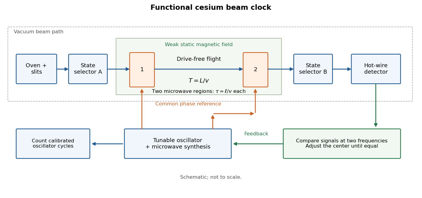
Here $F$ labels the total angular momentum and $m_F$ its projection. The selected pair is a two-level system inside a larger set of atomic energy levels; treating every oven atom as a prepared qubit would overstate the preparation. A measured detector signal may be modeled as $S(\nu )=S_{\mathrm{bg}}+A\overline{P}(2\pi ({\nu }_0-\nu ))$, with background $S_{\mathrm{bg}}$ and gain $A>0$. Background subtraction and stable transmission are necessary before interpreting the signal as a transition probability. The velocity-averaged Ramsey line provides one explicit ideal example; its chosen dimensions are not historical specifications.

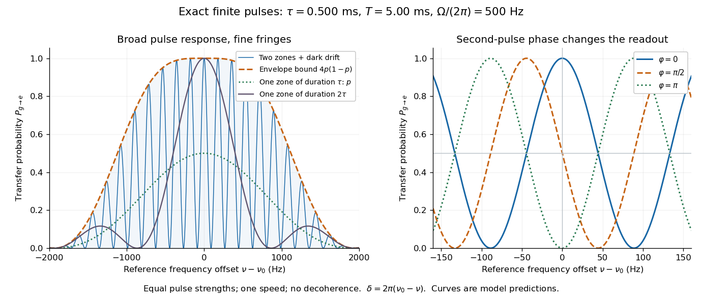
The exact finite-pulse Ramsey transition probability separates a slowly varying pulse response from rapid quantum interference. Define the single-zone transfer probability $p$ and a pulse-induced quantum phase $\theta$ bySince $c_p^2+b^2=1-p$, factorizing the real bracket in the original formula givesWhere $c_p=b=0$, the probability is zero and $\theta$ need not be defined. Elsewhere this identity proves the envelope bound without a weak-drive assumption. The envelope $4p(1-p)$ is not the single-zone response $p$: two equal coherent interactions have different transfer weights. A contiguous resonant Rabi pi pulse of duration $2\tau$ provides another useful comparison with the same total drive duration, but no dark interval. Its line is broad because it has no long flight phase.

Let each drive region have length $\ell$ and the drive-free gap have length $L$, measured edge to edge. A particle of constant speed $v>0$ experiences $\tau (v)=\ell /v$ and $T(v)=L/v$. For a normalized detected-beam speed probability density function $f(v)$, sum the transition probabilities, not the probability amplitudes of different particles:The displayed $f$ is an ideal effusion flux distribution, with speed scale $u$, uniform transmission and speed-independent detection efficiency. It is not a claim about any particular clock's selected beam. The substitution $x=(v/u{)}^2$ gives $f(v)dv=x{e}^{-x}dx$, proving normalization. Actual apertures, state selection and readout can change the effective weights.

For an original example choose $\ell =0.10\mathrm{m}$, $L=1.00\mathrm{m}$, $u=v_{\ast }=200\mathrm{m}{\mathrm{s}}^{-1}$ and $\Omega =2\pi \times 500\mathrm{rad}{\mathrm{s}}^{-1}$. The reference particle has ${\tau }_{\ast }=0.500\mathrm{ms}$, $T_{\ast }=5.00\mathrm{ms}$ and resonant $\pi /2$ pulses. The instantaneous-pulse width would be $100\mathrm{Hz}$. The exact finite-pulse width for that single speed is about $88.7\mathrm{Hz}$; the chosen distribution also reduces the on-resonance average to approximately $0.738$ because not every particle receives a $\pi /2$ pulse.

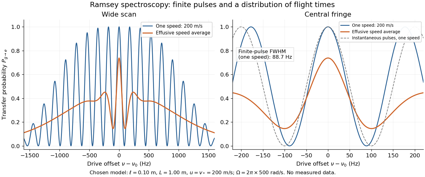
Different velocities smear side fringes because $\delta L/v$ varies across the beam. Nevertheless every term is even in $\delta$, so this symmetric ideal-model average has no odd line asymmetry that could displace the central lock point. Reduced contrast or altered width alone is not evidence of a shifted line center. A speed-dependent transition shift or unequal drive quantum phases changes that conclusion; atomic clock frequency shifts explains why these distinctions matter experimentally.