Finite-pulse Ramsey transition probability ($P_{g\to e}(\delta ;\tau ,T)$)

Use the Driven two-level Rabi model in the ordered basis $(|e⟩,|g⟩)$, with Pauli matrices satisfying ${\sigma }_z=\mathrm{diag}(1,-1)$. Let the Rabi detuning be $\delta ={\omega }_0-\omega =2\pi ({\nu }_0-\nu )$, in angular frequency, while ${\nu }_0$ and $\nu$ are ordinary frequencies in hertz. Assume two identical square pulses, equal drive oscillation phases, constant positive Rabi angular frequency $\Omega$, constant $\delta$ during pulses and flight, and no quantum decoherence or loss. The rotating-wave approximation and isolation of the chosen two-level system are required, just as for the Driven two-level Rabi model. Free flight means no transverse drive; the reference oscillator continues running.

The pulse and free-flight Hamiltonian operators in the rotating frame areThe Pauli matrix multiplication law gives $(\delta {\sigma }_z+\Omega {\sigma }_x{)}^2=q^{2}I$. Thus the exact special unitary group $\mathrm{SU}(2)$ pulse matrix for this effective Hamiltonian operator, and the flight matrix, areThe sequence is $U_p{U}_f{U}_p$. Starting in $|g⟩$, matrix multiplication and the Born rule giveThis retains the tilted rotation axis and quantum phase accumulated during each finite pulse. At resonance it gives $P_{g\to e}(0)={\sin }^2(\Omega \tau )$; with no flight it reduces to the single square-pulse response for duration $2\tau$. Both checks would fail if arbitrary ideal $\pi /2$ rotations were silently substituted at nonzero Rabi detuning.

For resonant pulse area $\Omega \tau =\pi /2$, $|\delta |/\Omega \ll 1$ and $\tau \ll T$, the central fringe approachesIts half-height points are $|\nu -{\nu }_0|=1/(4T)$, so the central peak's full width at half maximum is $1/(2T)$ in hertz, or $\pi /T$ in angular frequency. This width assumes an effectively flat pulse envelope across that central peak, one flight time and unit contrast; it is neither a universal finite-pulse width nor a frequency uncertainty. Longer flight lets a smaller frequency difference accumulate the same observable quantum phase.

The two pulses here have the same sign and the plotted outcome is transfer to $|e⟩$. The earlier Ramsey interferometry example uses an inverse analysis pulse and reports return to its initial label. Specifying the measured outcome and pulse oscillation phases reconciles the two conventions. In a beam the lengths and speed determine $\tau$ and $T$; in the Quantronium Ramsey interference experiment electronics set the pulse times for a stationary circuit.

The exact finite-pulse Ramsey transition probability separates a slowly varying pulse response from rapid quantum interference. Define the single-zone transfer probability $p$ and a pulse-induced quantum phase $\theta$ bySince $c_p^2+b^2=1-p$, factorizing the real bracket in the original formula givesWhere $c_p=b=0$, the probability is zero and $\theta$ need not be defined. Elsewhere this identity proves the envelope bound without a weak-drive assumption. The envelope $4p(1-p)$ is not the single-zone response $p$: two equal coherent interactions have different transfer weights. A contiguous resonant Rabi pi pulse of duration $2\tau$ provides another useful comparison with the same total drive duration, but no dark interval. Its line is broad because it has no long flight phase.

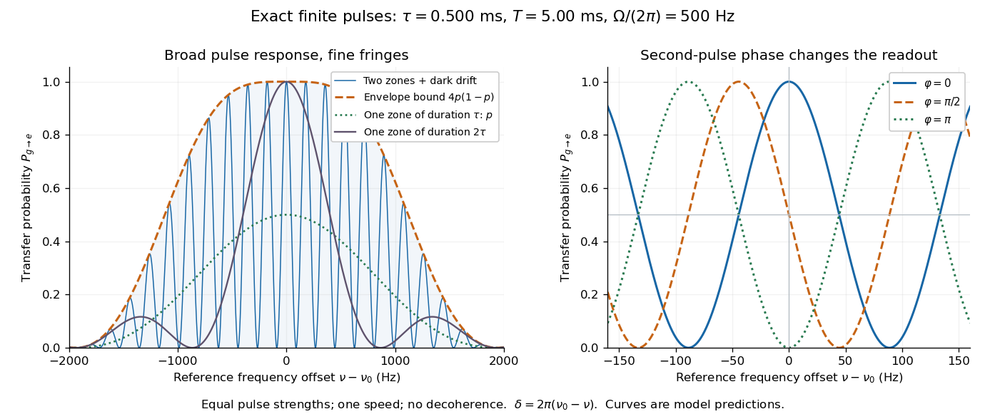
Keep the first pulse's oscillation phase zero and give the second phase $\phi$ in the Driven two-level Rabi model. Its upper off-diagonal Hamiltonian operator entry is $\hslash \Omega e^{-i\phi }/2$. Multiplying the two pulse unitary operators and the free-flight unitary operator givesThe Born rule gives the displayed phase-dependent form using the $p,b,\theta$ of the Ramsey fringe envelope. Thus $\phi =0$ reproduces the existing expression, while $\phi =\pi$ turns a resonant transfer maximum into zero transfer. A single pulse's population is insensitive to its drive phase; the second coherent interaction makes their difference observable. An uncontrolled, uniformly random $\phi$ instead averages this probability to $2p(1-p)$, leaving the broad pulse response but removing the dark-flight fringes.

Finite pulses also contribute to the near-resonant frequency slope. For $\Omega \tau =\pi /2$, differentiating $\theta$ at $\delta =0$ gives ${\theta }^{\prime }(0)=1/\Omega$. Consequently the phase near resonance isAt $\phi =\pi /2$ the exact resonant slope is $\partial P/\partial \nu =-\pi T_{\mathrm{eff}}$. For the plotted parameters $T_{\mathrm{eff}}\simeq 5.637\mathrm{ms}$; the near-resonant estimate $1/(2T_{\mathrm{eff}})\simeq 88.71\mathrm{Hz}$ explains why the exact finite-pulse width below differs from $100\mathrm{Hz}$. The slope is exact at resonance under these assumptions, while this width estimate uses the local phase expansion. A velocity distribution requires averaging the full response, not substituting one effective flight time.

Let each drive region have length $\ell$ and the drive-free gap have length $L$, measured edge to edge. A particle of constant speed $v>0$ experiences $\tau (v)=\ell /v$ and $T(v)=L/v$. For a normalized detected-beam speed probability density function $f(v)$, sum the transition probabilities, not the probability amplitudes of different particles:The displayed $f$ is an ideal effusion flux distribution, with speed scale $u$, uniform transmission and speed-independent detection efficiency. It is not a claim about any particular clock's selected beam. The substitution $x=(v/u{)}^2$ gives $f(v)dv=x{e}^{-x}dx$, proving normalization. Actual apertures, state selection and readout can change the effective weights.

For an original example choose $\ell =0.10\mathrm{m}$, $L=1.00\mathrm{m}$, $u=v_{\ast }=200\mathrm{m}{\mathrm{s}}^{-1}$ and $\Omega =2\pi \times 500\mathrm{rad}{\mathrm{s}}^{-1}$. The reference particle has ${\tau }_{\ast }=0.500\mathrm{ms}$, $T_{\ast }=5.00\mathrm{ms}$ and resonant $\pi /2$ pulses. The instantaneous-pulse width would be $100\mathrm{Hz}$. The exact finite-pulse width for that single speed is about $88.7\mathrm{Hz}$; the chosen distribution also reduces the on-resonance average to approximately $0.738$ because not every particle receives a $\pi /2$ pulse.

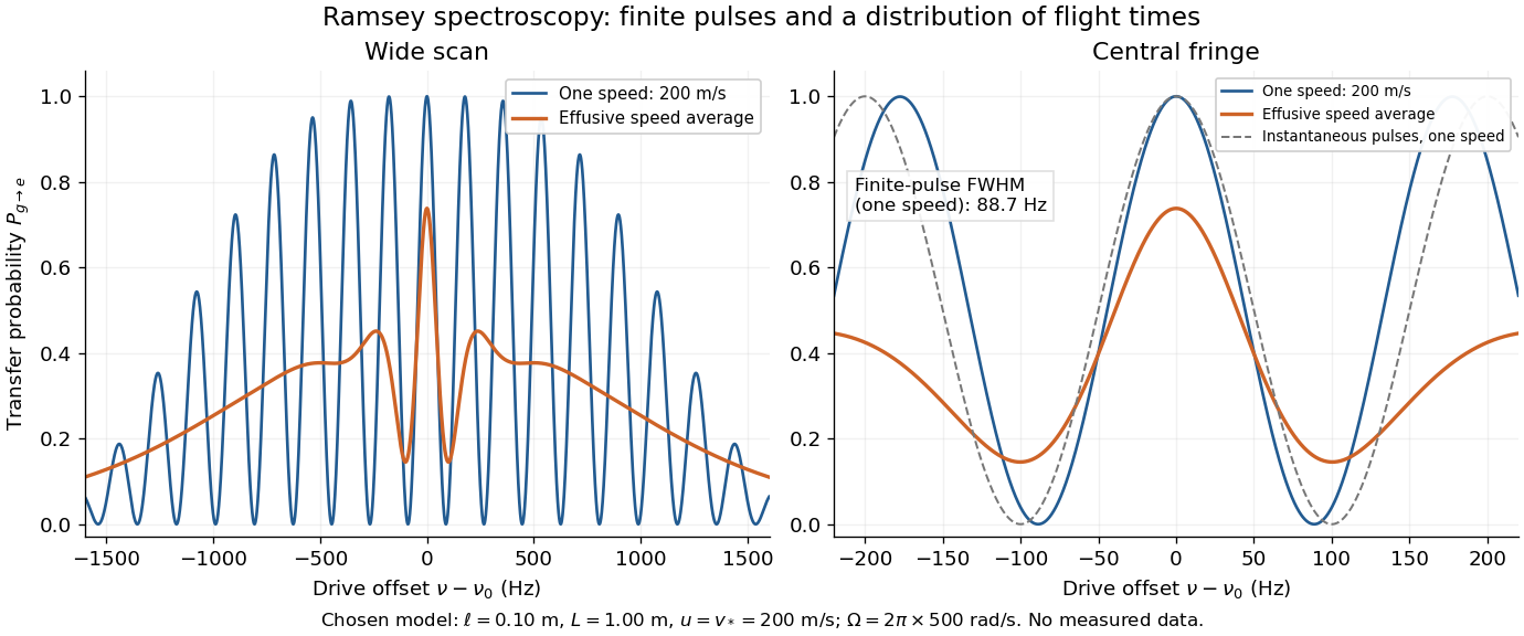
Different velocities smear side fringes because $\delta L/v$ varies across the beam. Nevertheless every term is even in $\delta$, so this symmetric ideal-model average has no odd line asymmetry that could displace the central lock point. Reduced contrast or altered width alone is not evidence of a shifted line center. A speed-dependent transition shift or unequal drive quantum phases changes that conclusion; atomic clock frequency shifts explains why these distinctions matter experimentally.