Consult Apexshield Recovery if you have been a victim of any online crypto related scam.They are open to help you recover that Bitcoin,usdt and wallet which you have lost in the past.
I am sharing this here because I have been a victim of an online investment scam and I understand how it feels to lose a huge amount of money to a scam. I am immensely grateful to Apexshield Recovery for their exceptional service and I would highly recommend reaching out to Apexshield Recovery via Google , to anyone who wants to recover scammed bitcoin, stolen cryptocurrency, funds lost to binary options forex, funds lost to fake online investment and any other form of online scam for consultation and assistance . Their professionalism, expertise, and commitment to customer satisfaction truly set them apart. Search "Apexshield Recovery" or reachout to them through their contact information below.
I am sharing this here because I have been a victim of an online investment scam and I understand how it feels to lose a huge amount of money to a scam. I am immensely grateful to Apexshield Recovery for their exceptional service and I would highly recommend reaching out to Apexshield Recovery via Google , to anyone who wants to recover scammed bitcoin, stolen cryptocurrency, funds lost to binary options forex, funds lost to fake online investment and any other form of online scam for consultation and assistance . Their professionalism, expertise, and commitment to customer satisfaction truly set them apart. Search "Apexshield Recovery" or reachout to them through their contact information below.
Welcome to my home page!
Hinged Unloader Knee Brace: Complete Guide to Pain Relief and Knee Support by  z1knee knee brace 0 2026-07-10
z1knee knee brace 0 2026-07-10Knee pain can make everyday activities such as walking, climbing stairs, exercising, or even standing for long periods uncomfortable. Whether the discomfort is caused by osteoarthritis, ligament instability, or uneven pressure within the knee joint, wearing the right brace can make a significant difference. A hinged unloader knee brace is specifically designed to provide stability while shifting pressure away from the damaged side of the knee.
Unlike standard compression sleeves, this brace combines a rigid hinged frame with unloading technology to improve alignment, reduce joint stress, and promote more comfortable movement. It is widely recommended for people who want to remain active while managing chronic knee pain.
In this guide, we'll explain how a hinged unloader knee brace works, who should wear one, its benefits, limitations, and what to consider before purchasing.
What Is a Hinged Unloader Knee Brace?
A hinged unloader knee brace is an orthopedic support designed to reduce pressure on one side of the knee while maintaining stability during movement.
A hinged unloader knee brace is an orthopedic support designed to reduce pressure on one side of the knee while maintaining stability during movement.
The brace includes:
Strong metal or aluminum side hinges
Adjustable unloading mechanism
Comfortable straps for a customized fit
Cushioned pads for pressure distribution
Lightweight frame for daily use
The hinges help control knee motion, while the unloading system gently shifts body weight away from the damaged compartment of the knee.
Adjustable unloading mechanism
Comfortable straps for a customized fit
Cushioned pads for pressure distribution
Lightweight frame for daily use
The hinges help control knee motion, while the unloading system gently shifts body weight away from the damaged compartment of the knee.
This combination makes it especially useful for individuals experiencing pain due to unicompartmental knee osteoarthritis or instability.
How Does a Hinged Unloader Knee Brace Work?
The brace applies a controlled corrective force known as a three-point pressure system.
The brace applies a controlled corrective force known as a three-point pressure system.
Here's how it functions:
Supports the knee joint with rigid side hinges.
Applies gentle corrective pressure.
Shifts body weight away from the painful side.
Reduces bone-on-bone contact.
Improves knee alignment.
Allows smoother movement with less discomfort.
Instead of placing equal pressure across the entire knee, the brace redistributes the load, helping decrease pain during walking and standing.
Conditions That May Benefit From a Hinged Unloader Knee Brace
A doctor may recommend this type of brace for several knee conditions, including:
A doctor may recommend this type of brace for several knee conditions, including:
Knee Osteoarthritis
One of the most common reasons for using an unloader brace is medial or lateral compartment osteoarthritis.
One of the most common reasons for using an unloader brace is medial or lateral compartment osteoarthritis.
It helps reduce pressure on the worn cartilage, allowing more comfortable movement.
Mild Ligament Instability
The hinged design provides additional support when the knee feels unstable due to previous ligament injuries.
The hinged design provides additional support when the knee feels unstable due to previous ligament injuries.
Meniscus Degeneration
People with degenerative meniscus problems may benefit from reduced compartment loading.
People with degenerative meniscus problems may benefit from reduced compartment loading.
Post-Surgical Recovery
In some rehabilitation programs, doctors may recommend an adjustable hinged brace to protect healing tissues.
In some rehabilitation programs, doctors may recommend an adjustable hinged brace to protect healing tissues.
Always follow your healthcare provider's advice regarding post-operative brace use.
Benefits of a Hinged Unloader Knee Brace
Reduces Knee Pain
By unloading the damaged side of the knee, the brace often decreases pain during daily activities.
Reduces Knee Pain
By unloading the damaged side of the knee, the brace often decreases pain during daily activities.
Improves Stability
The rigid hinges help control unwanted knee movement, providing extra confidence while walking.
The rigid hinges help control unwanted knee movement, providing extra confidence while walking.
Supports Natural Movement
Unlike rigid immobilizers, hinged braces allow controlled bending and extension.
Unlike rigid immobilizers, hinged braces allow controlled bending and extension.
Helps Delay Surgery
For some individuals with osteoarthritis, conservative treatments such as an unloader brace may help postpone surgical intervention.
For some individuals with osteoarthritis, conservative treatments such as an unloader brace may help postpone surgical intervention.
Encourages Physical Activity
Reduced pain often makes it easier to participate in walking programs, physical therapy, and low-impact exercise.
Reduced pain often makes it easier to participate in walking programs, physical therapy, and low-impact exercise.
Adjustable Compression
Most models allow users to modify strap tension for better comfort and support.
Most models allow users to modify strap tension for better comfort and support.
Individuals with medial knee osteoarthritis
People with lateral compartment arthritis
Adults experiencing uneven knee joint loading
Patients recovering under medical supervision
Active individuals seeking additional knee stability
Those wishing to remain mobile while managing chronic knee pain
A proper evaluation by an orthopedic specialist is recommended before choosing an unloading brace.
Who Should Not Use One Without Medical Advice?
Although these braces are helpful, they are not appropriate for everyone.
Although these braces are helpful, they are not appropriate for everyone.
Consult your healthcare provider if you have:
Severe knee deformities
Advanced ligament tears requiring surgery
Significant swelling
Skin infections around the knee
Circulation disorders
Poor brace tolerance due to other medical conditions
Features to Look for in a Hinged Unloader Knee Brace
Choosing the right brace improves comfort and effectiveness.
Advanced ligament tears requiring surgery
Significant swelling
Skin infections around the knee
Circulation disorders
Poor brace tolerance due to other medical conditions
Features to Look for in a Hinged Unloader Knee Brace
Choosing the right brace improves comfort and effectiveness.
Consider these features:
Adjustable Hinges
Allow customized support based on your condition.
Allow customized support based on your condition.
Lightweight Frame
Makes prolonged wear more comfortable.
Makes prolonged wear more comfortable.
Breathable Materials
Help reduce sweating during extended use.
Help reduce sweating during extended use.
Secure Strap System
Keeps the brace stable throughout daily activities.
Keeps the brace stable throughout daily activities.
How to Measure for the Correct Size
Proper sizing is essential.
Proper sizing is essential.
Typically, measurements include:
Thigh circumference
Knee circumference
Calf circumference
Always compare your measurements with the manufacturer's sizing chart rather than choosing based solely on clothing size.
Knee circumference
Calf circumference
Always compare your measurements with the manufacturer's sizing chart rather than choosing based solely on clothing size.
Wear the brace directly against clean, dry skin or over a thin sleeve if recommended.
Align the hinges with the center of the knee.
Fasten straps from bottom to top.
Tighten evenly without restricting circulation.
Walk for a few minutes and readjust if necessary.
Improper positioning can reduce effectiveness.
Align the hinges with the center of the knee.
Fasten straps from bottom to top.
Tighten evenly without restricting circulation.
Walk for a few minutes and readjust if necessary.
Improper positioning can reduce effectiveness.
Can You Wear It Every Day?
Many users wear a hinged unloader knee brace daily, particularly during activities that place stress on the knee.
Many users wear a hinged unloader knee brace daily, particularly during activities that place stress on the knee.
Common activities include:
Walking
Grocery shopping
Yard work
Standing for long periods
Light exercise
Physical therapy
Wear duration should follow your healthcare provider's recommendations.
Grocery shopping
Yard work
Standing for long periods
Light exercise
Physical therapy
Wear duration should follow your healthcare provider's recommendations.
Can You Exercise While Wearing It?
Yes, many low-impact activities are possible while wearing the brace, including:
Yes, many low-impact activities are possible while wearing the brace, including:
Walking
Stationary cycling
Elliptical training
Physical therapy exercises
Light hiking
Strengthening exercises
Avoid high-impact sports unless approved by your healthcare professional.
Stationary cycling
Elliptical training
Physical therapy exercises
Light hiking
Strengthening exercises
Avoid high-impact sports unless approved by your healthcare professional.
Tips include:
Clean straps regularly.
Wipe hinges with a damp cloth.
Air dry completely.
Inspect screws and hinges periodically.
Replace worn straps if needed.
Store in a cool, dry place.
Avoid machine washing unless the manufacturer specifically allows it.
Wipe hinges with a damp cloth.
Air dry completely.
Inspect screws and hinges periodically.
Replace worn straps if needed.
Store in a cool, dry place.
Avoid machine washing unless the manufacturer specifically allows it.
Avoid:
Wearing the wrong size
Overtightening straps
Wearing the brace too loosely
Ignoring alignment instructions
Skipping follow-up adjustments
Continuing use despite increasing pain without consulting a doctor
Hinged Unloader Knee Brace vs Standard Hinged Knee Brace
Feature Hinged Unloader Knee Brace Standard Hinged Knee Brace
Unloads knee compartment ✔ Yes ✖ No
Knee stability ✔ Excellent ✔ Good
Osteoarthritis support ✔ Excellent Limited
Ligament protection ✔ Yes ✔ Yes
Adjustable unloading ✔ Yes Usually No
Daily walking comfort Excellent Good
Frequently Asked Questions
Does a hinged unloader knee brace cure arthritis?
No. It helps manage symptoms by reducing pressure on the affected part of the knee but does not reverse arthritis.
Can I wear it under clothing?
Many low-profile designs fit under loose-fitting pants, though bulkier models may be noticeable.
Many low-profile designs fit under loose-fitting pants, though bulkier models may be noticeable.
Will it replace knee surgery?
Not necessarily. It is a conservative treatment option that may help reduce symptoms and improve function, but some people may still require surgery depending on the severity of their condition.
Not necessarily. It is a conservative treatment option that may help reduce symptoms and improve function, but some people may still require surgery depending on the severity of their condition.
How long does it take to get used to wearing one?
Most users adapt within a few days to a couple of weeks, depending on the fit and the amount of time the brace is worn.
Most users adapt within a few days to a couple of weeks, depending on the fit and the amount of time the brace is worn.
Is it suitable for both knees?
Yes. Many models are available for both left and right knees, though you should select the correct version and fit for the affected side.
Yes. Many models are available for both left and right knees, though you should select the correct version and fit for the affected side.
Conclusion
A hinged unloader knee brace offers an effective non-surgical solution for people experiencing knee pain caused by osteoarthritis, joint misalignment, or mild instability. By combining rigid hinged support with unloading technology, it reduces pressure on the affected compartment of the knee while allowing controlled, natural movement.
A hinged unloader knee brace offers an effective non-surgical solution for people experiencing knee pain caused by osteoarthritis, joint misalignment, or mild instability. By combining rigid hinged support with unloading technology, it reduces pressure on the affected compartment of the knee while allowing controlled, natural movement.
When properly fitted and used as part of a comprehensive treatment plan that may include physical therapy, exercise, and weight management, a hinged unloader knee brace can help improve comfort, increase mobility, and support an active lifestyle. Before purchasing one, consult a healthcare professional to ensure the brace is appropriate for your specific condition and fitted correctly for the best possible results.
Welcome to my home page!
Puzzle games are a great way to relax while still giving your brain something fun to do. One of the most interesting word-based puzzle experiences is Connections Game, a game that challenges you to spot hidden relationships between words. It looks simple at first, but the deeper you play, the more you realize how clever and surprising it can be.
connectionsgamefree.com
The basic idea is to group words that share a common connection. These connections may be based on meaning, category, wordplay, pop culture, phrases, or even subtle associations. This makes every round feel like a small mystery to solve.
connectionsgamefree.com
The basic idea is to group words that share a common connection. These connections may be based on meaning, category, wordplay, pop culture, phrases, or even subtle associations. This makes every round feel like a small mystery to solve.
In Connections Game, you are usually given a grid of words. Your task is to divide them into several groups, with each group containing words that belong together in some way. For example, one group might contain types of fruit, while another could include words often used in movie titles.
The fun comes from figuring out which words fit together and which ones are meant to mislead you. Some words may seem like they belong in one category but actually fit better somewhere else. This creates a satisfying challenge where you need to think carefully before making a choice.
To play, read through all the words first. Try to identify any obvious categories, then look for less direct connections. Once you think you have a complete group, select those words and submit your guess. If you are correct, that group is cleared, helping you focus on the remaining words.
Tips for Better Play
One helpful tip is to avoid rushing. Connections often rewards patience more than speed. Take a moment to say the words out loud or think about different meanings they might have. A word can sometimes be a noun, verb, name, brand, or part of a common phrase.
Another useful strategy is to look for traps. If three words seem clearly connected but you cannot find a fourth, the game may be guiding you toward a false match. Step back and consider other possibilities.
It also helps to start with the most obvious group. Clearing one category can make the rest of the puzzle easier. After that, focus on unusual words, because they often point toward the theme of a hidden group.
If you get stuck, take a short break. Coming back with fresh eyes can make a connection suddenly stand out. This is one reason the Connections Game is enjoyable for casual play: you can spend a few minutes on it or take your time without pressure.
Conclusion
Connections Game is easy to learn but full of clever surprises. It combines vocabulary, logic, memory, and lateral thinking in a way that feels both relaxing and rewarding. Whether you enjoy word puzzles every day or just want a quick mental challenge, it offers a simple format with plenty of depth.
The best way to experience it is to stay curious, be patient, and enjoy the small “aha” moments when a hidden category finally makes sense.
Welcome to my home page!
Are you looking for a beautiful and sexy young girl tonight in Noida? If your answer is yes, then our cheap Noida call girls are always eager to be with you in your place. Whether it’s a hotel or home, for a wonderful experience, they can be your real girlfriend as well as play any role to bring excitement to the sex session.
Verified females are educated and well-trained to be your companions and night partners. Whether you need a Noida cheap call girls for a date, business meetings, or a movie date. We are the best choice for these situations and for pleasure. These ultra-sexy best Call Girls in Noida are beyond imagination on different occasions and events.
There is nothing that our seductive and delightful girls can’t provide in one session. Our call girl in Noida is available 24/7 to ensure your pleasure. Similarly, our cheap call girls are gaining more attention in the entertainment sector. Our beautiful Noida Call Girls are here to make unforgettable memories in the bustling city. So don’t miss this opportunity to spend time with our Young and mature housewife call girls in Noida.
Experience The Top Rated Noida cheap call girls Near me with 100% Safe Call Girls in Noida
Hello Gentlemen, Welcome to Noida, the capital of India. Noida is a dynamic city that has melded with dynamic future vision. A mix of markets, offices, clubs, hotels, and a busy business hub. With an abundant array of opportunities for creativity and advancement, Noida attracts every person who wants to achieve their goals and dreams on the grandest scale possible. If you are one of those who have adult and sensual desires.
Hello Gentlemen, Welcome to Noida, the capital of India. Noida is a dynamic city that has melded with dynamic future vision. A mix of markets, offices, clubs, hotels, and a busy business hub. With an abundant array of opportunities for creativity and advancement, Noida attracts every person who wants to achieve their goals and dreams on the grandest scale possible. If you are one of those who have adult and sensual desires.
Now you want to make them come true with a hot and sexy Noida cheap call girls. Then dear, today you are at the right destination. Here you can meet with your desired girls and can fulfill your all sexual fantasies. Meet our Noida cheap call girl girls who are completely ready to provide you with next-level service and adult entertainment. We will provide you memorable moments of your life. That you will never forget, choose your pretty girls with those you want feel like heaven.
Most Reliable and Trusted Noida cheap Girls Only in Rs 4999 Book Now
Our Noida call girl Service has become the most important part of every erotic night spent. Our verified cheap call girl Girls in Noida are available for booking 24/7 in the city. Whether you need a young and charming girl in your house or at lavish hotels. Our female companion in Noida will reach you as soon as possible.
Our Noida call girl Service has become the most important part of every erotic night spent. Our verified cheap call girl Girls in Noida are available for booking 24/7 in the city. Whether you need a young and charming girl in your house or at lavish hotels. Our female companion in Noida will reach you as soon as possible.
This is our commitment to our valued customers. Furthermore, you can expect all erotic solutions and deep pleasure from our ladies. They are born to satisfy and entertain clients with their stunning figures and attractive nature.
Spending a night with a sexy cheap Call Girls in Noida is a boon for any man. If you want to experience a memorable night with your favorite partner, then this is an effective solution to schedule a romantic night together. The sensual companions in Noida are waiting for your call. Call us to schedule a meeting with these hotties.
hi.vipnoidacallgirl.in/
hi.vipnoidacallgirl.in/
Welcome to my home page!
☎️+2347073791700☎️ I WANT TO JOIN ILLUMINATI SOCIETY FOR MONEY RITUAL by zozumuhah35 0 2026-07-09 2026-07-09
zozumuhah35 0 2026-07-09 2026-07-09+2349065144043 HERE IN ZOZUMUHAH BROTHERHOOD WE BELIEVE IN POWER,FAME, PROTECTION, OFFICE PROMOTION, POLITICAL AMBITION AND ENDLESS WEALTH INTERESTED ONES SHOULD CONTACT THE TEMPLE GRANDMASTERS @+2349065144043
DO YOU WANT TO JOIN OCCULT OF BILLIONAIRES TO BE WELL KNOWN AND POWERFUL FOR MONEY AND PROTECTION HERE IN NIGERIA AND GHANA CALL US ON +2349065144043 or email zozumuhahbrotherhood@gmail.com You were born free and will die free someday, but will you live free? As long as habit and routine dictate the pattern of living, new dimensions of the soul will not emerge. JOIN our powerful society to gain and practice secret knowledge and information that was once only accessible by the privileged elite and society members.This is a private, exclusive, members-only global association.+2347073791700 No matter how much the rich have, they always want more. And the richer you are, the more you get. And the more you get, the less others get, so you are actively making the poor poorer. Isn't that the world we live in? That's how we have the 1% versus the 99%. They will take everything from us, unless we take it all back from them. The difference between a successful person and others is not a lack of strength, not a lack of knowledge, but rather a lack of will. Get off the poverty road and onto the path of prosperity now. If money has been tight and things haven’t been going very well financially, Our ZOZUMUHAHBROTHERHOOD society will empower you to change your life and live your life to the fullest, success belongs to those who do something to change there world +2349065144043 WHY SUFFER IN POVERTY WHEN YOU CAN JOIN ZOZUMUHAHBROTHERHOOD AND BECOME MILLIONAIRE INSTANTLY WHY SEARCHING FOR POWER AT THE WRONG PLACE. WHEN THERE IS GREATEST OF ALL IN UNIVERSE. GET YOUR POWER FROM ZOZUMUHAH BROTHERHOOD. IS THE GREATEST OCCULT.TO JOIN US CALL THE WISE ONE ON THIS NUMBER +2349065144043 WELCOME TO OUR OFFICIAL SITE TO JOIN US.OUR END OF THE YEAR INITIATION CEREMONY IS COMING SOON AND WE WANT TO USE THIS OPPORTUNITY TO TELL YOU THAT YOU ARE ENTITLE AND WELCOME TO ZOZUMUHAH BROTHERHOOD OCCULT WE MADE YOU RICH, BECAUSE WE RULE THE WORLD WITH OUR GREAT POWER AND THE NEW WORLD ORDER.THE DOOR IS OPEN TO NEW SPECIES TO JOIN, THIS IS A GOLDEN OPPORTUNITY. JOIN ZOZUMUHAHBROTHERHOOD OCCULT SOCIETY NOW,GET WHAT IS YOUR FAITHFUL DESIRES,FAME,WEALTH,MONEY,POPULARITY,QUICK MONEY,MAGIC RING,HERBS AND POWER.. WE ARE THE GREAT ZOZUMUHAH BROTHERHOOD WHICH BEING SEND BY OUR LORD SPIRITUAL .JOIN US NOW TO EXPERIENCE OUR POWER IN YOUR HAND,THE POWER OF THE SUN!IS IN MY HAND..THE BENEFIT GIVEN TO NEW MEMBERS IS UNFORGETTABLE GIFT,JOIN US AND BECOME RICH IN JUST FEW DAYS AFTER YOUR INITIATION +2349065144043 BE SURE YOU HAVE MAKE UP YOUR MIND, BEFORE CONTACTING US REGARDING ANY ISSUE, WE ARE NOT HERE FOR CHILD'S PLAY, THE ZOZUMUHAHBROTHERHOOD BASE ON ANIMAL SACRIFICE AND NO HUMAN BLOOD IS INVOLVE, JOIN US TODAY AND BE WEALTHY AND FAMOUS AND SHAKE HANDS WITH OUR LORD SABANTAI THE GODS OF WEALTH AND RICHES. FOR MORE INFORMATION AND ENQUIRERS CALL +2349065144043 or you can email us on zozumuhahbrotherhood@gmail.com ALL ZOZUMUHAH BROTHERHOOD INITIATE MEMBERS ARE ENTITLED TO EVERYTHING THAT MAKE LIFE WORTH LIVING,NO MATTER HOW EXPENSIVE IT'S MIGHT BE, CARS,HOUSES, LUXURIOUS LIFE,BUT ONE THING YOU MUST PUT FIRST IS COURAGE AND BRAVERY BECAUSE THOSE ARE THE KEYS TO UNLOCK TO ONE FORTUNE, AND BEFORE ANY MAN/WOMAN CAN BE ACCEPTED HERE HE OR SHE IS EXPECTED TO HAVE MADE UP HIS OR HER KNOWING THE TASK AHEAD, THOUGH WE DON'T USE HUMAN BLOOD FOR SACRIFICE BUT DO NOT BE DECEIVED; WE USE ANIMAL BLOOD TO PLEASE THE LORD, GUARDIANS OF AGE TO ACCEPT YOU AFTER WHICH YOU'LL BE ENDOWED WITH RICHES AND LUXURY,BUT KNOW THAT THERE'S GRAND PRICE TO PAY WHICH IS OFFERING YOUR SOUL TO THE LORD LUCIFER AT A CERTAIN STAGE (80YEARS) ................ NOTHING ELSE WILL BE REQUIRED UNTIL YOUR LST SACRIFICIAL RITE AND MONEY WILL NOT BE YOUR PROBLEM AGAIN UNTIL YOU DIE. WHAT EVER PROBLEM YOU HAVE ZOZUMUHAH BROTHERHOOD HAVE ALL IT'S TAKES TO MAKE THAT MAN/WOMAN YOU WISH TO BECOME ITS IS NOT BAD TO BE BORN IN A POOR BACKGROUND BUT YOU WILL MAKE HUGE MISTAKE WHEN YOU ALLOW YOURSELF TO DIE WITHOUT MAKING YOUR DREAMS COME TRUE,......
POVERTY IS A DECEASE THAT SOMETIMES GET INTO YOUR HEAD AND DESTROY THAT BEAUTIFUL DREAMS YOU HAVE ALWAYS HAD, TODAY ZOZUMUHAH BROTHERHOOD IS HERE TO END IT HERE WE SEND POVERTY TO EXCEIL WHERE ITS WOULDN'T RETURN AGAIN
TAKE THIS OPPORTUNITY TODAY AND TURN YOUR LIFE AROUND FOR GOOD MIND YOU NO HUMAN BLOOD IS NEEDED TO FULLFIL YOUR DREAMS IT'S CAN ONLY TAKE YOU FEW ASSIGNMENT TO POSES POWER HERE IN ZOZUMUHAH BROTHERHOOD CALL FOR YOUR INITIATION +2349065144043 OR EMAIL zozumuhahbrotherhood@gmail.com NO PROBLEM WITHOUT SOLUTION .... ...
Welcome to my home page!
The foundation of every powerful computer vision system lies in the precision of its training data. Without accurate labeling, machine learning models struggle to understand spatial dimensions, identify objects, or safely navigate real-world environments. To achieve dependable machine intelligence, businesses require meticulously labeled imagery.
The Role of Accurate Labeling in AI Success
Building robust computer vision applications demands flawless datasets. Utilizing specialized Image annotation services ensures that every image is precisely marked using techniques like semantic segmentation, bounding boxes, and polygon mapping. This foundational accuracy is essential for eliminating algorithmic bias, reducing errors, and training highly reliable models.
Building robust computer vision applications demands flawless datasets. Utilizing specialized Image annotation services ensures that every image is precisely marked using techniques like semantic segmentation, bounding boxes, and polygon mapping. This foundational accuracy is essential for eliminating algorithmic bias, reducing errors, and training highly reliable models.
Scale Your Operations with Expert Assistance
Managing large-scale data annotation internally can strain valuable time and engineering resources. Leveraging external Image annotation services allows development teams to seamlessly scale their training pipelines, achieve superior data quality, and significantly reduce time-to-market.
Managing large-scale data annotation internally can strain valuable time and engineering resources. Leveraging external Image annotation services allows development teams to seamlessly scale their training pipelines, achieve superior data quality, and significantly reduce time-to-market.
Visit to get Image annotation services: annotationbox.com/image-annotation-services/
Welcome to my home page!
Welcome to my home page!

Welcome to my home page!
Welcome to my home page!
Welcome to my home page!

Welcome to my home page!
◌🅯◌᯽◌🅯◌𖡗◌🅯◌᯽◌🅯◌⚪◌🅯◌᯽◌🅯◌𖡗◌🅯◌᯽◌🅯◌⠀◌🅯◌᯽◌🅯◌𖡗◌🅯◌᯽◌🅯◌⚪◌🅯◌᯽◌🅯◌𖡗◌🅯◌᯽◌🅯◌𖡗𔗢𖡗᯽𖡗𔗢𖡗 𖡗𔗢𖡗᯽𖡗𔗢𖡗◌🅯◌᯽◌🅯◌𖡗◌🅯◌᯽◌🅯◌⚪◌🅯◌᯽◌🅯◌𖡗◌🅯◌᯽◌🅯◌⠀◌🅯◌᯽◌🅯◌𖡗◌🅯◌᯽◌🅯◌⚪◌🅯◌᯽◌🅯◌𖡗◌🅯◌᯽◌🅯◌ by  𔗢᯽𔗢 𔗢᯽𔗢 0 2026-06-25
𔗢᯽𔗢 𔗢᯽𔗢 0 2026-06-25⠀
⚪𖡗⚪𖡼⚪𖡗⚪𔗢⚪𖡗⚪𖡼⚪𖡗⚪
◦୦◦◯◦୦◦⠀ ⠀◦୦◦◯◦୦◦
⚪𖡗⚪𖡼⚪𖡗⚪𔗢⚪𖡗⚪𖡼⚪𖡗⚪
𔗢᯽𔗢 𔗢᯽𔗢
⚪𖡗⚪𖡼⚪𖡗⚪𔗢⚪𖡗⚪𖡼⚪𖡗⚪
◦୦◦◯◦୦◦⠀ ⠀◦୦◦◯◦୦◦
⚪𖡗⚪𖡼⚪𖡗⚪𔗢⚪𖡗⚪𖡼⚪𖡗⚪
⠀
TϽUᗡTϽATЯƎTИIИMO 𔗢 OMNINTERTACTDUCT
ϱwji-h-httq-yo-t-r-f-202-0419-0214-2-httq-r-ar-h-it-44-mu-um-by-b\muɘƨum\Ԑ44:ɘtiƨ.hↄraɘƨɘr\\:ƨqtth\4ਟ-14ਟ1-9140-მ202\fɘr\ϽT.OYꓨ\\:qtth ◌𖡹◌🅯◌𖡹◌⚪◌𖡹◌🅯◌𖡹◌⠀◌𖡹◌🅯◌𖡹◌⚪◌𖡹◌🅯◌𖡹◌ GYO.TC/ref/2026-0419-1541-54/https://research.site:443/museum/d-yd-mu-um-44-ti-h-ra-r-qtth-2-4120-9140-202-f-r-t-oy-qtth-h-ijwg
7ɘმb8ↄ82Ԑbਟ2-ਟԐ08-92Ԑ4-ↄ7dↄ-72ਟↄ0ɘb4\ƨ\Ԑ44:ia.nɘwq.tahↄ\\:ƨqtth\01-2ਟმ0-მ2ਟ0-მ202\fɘr\ϽT.OYꓨ\\:qtth 🅯𖡗⚪𖡗🅯⠀🅯𖡗⚪𖡗🅯 GYO.TC/ref/2026-0526-0652-10/https://chat.qwen.ai:443/s/4de0c527-cb7c-4329-8035-25d328c8d6e7
lmth.latƨyrↄ\OꟻИI.ИƎЯᗡ⅃IHϽЯATƧ\_fi94844142ਟ0მ202\dɘw\ϱro.ɘvihↄra.dɘw\41-2122-ਟ2ਟ0-მ202\fɘr\ϽT.OYꓨ\\:qtth 𖡹🅯𖡹⠀𖡹🅯𖡹 GYO.TC/ref/2026-0525-2212-14/web.archive.org/web/20260524144849if_/STARCHILDREN.INFO/crystal.html
OIᗡUTƧƎƧЯƎVƎЯUTUꟻ@\MOϽ.ƎᗺUTUOY\ꓨЯO.ƎVIHϽЯA.ᗺƎW\\:ƨqtth 𖢒᳀𖢒⚪𖢒᳀𖢒⠀𖢒᳀𖢒⚪𖢒᳀𖢒 WEB.ARCHIVE.ORG/YOUTUBE.COM/@FUTUREVERSESTUDIO
lmth.qma𝼃jiɘrꞰ_ƨɘirᗡ\i𝼃iw\Ԑ44:ln.ƨrɘnowɘblob.www\\:ƨqtth\21-41Ԑ2-42ਟ0-მ202\fɘr\ϽT.OYꓨ\\:qtth ◯🅯◯⚪◯🅯◯⠀◯🅯◯⚪◯🅯◯ GYO.TC/ref/2026-0524-2314-12/https://www.bolbewoners.nl:443/wiki/Dries_Kreijkamp.html
ᗺA%4Ͻ%ƨ18%4Ͻ%va𝼃an18%4Ͻ%htƧ\i𝼃iw\Ԑ44:ϱro.aibɘqi𝼃iw.nɘ\\:ƨqtth\12-8ਟ12-ਟ090-ਟ202\fɘr\ϽT.OYꓨ\\:qtth 🅯⚪🅯⠀🅯⚪🅯 GYO.TC/ref/2025-0905-2158-21/https://en.wikipedia.org:443/wiki/Sth%C4%81nakav%C4%81s%C4%AB
მმ8Ԑ7ԐԐ4Ԑ1=biblo&noitↄnuf_ƨuidaꟻ=ɘltit?qhq.xɘbni\w\Ԑ44:ϱro.aibɘqi𝼃iw.nɘ\\:ƨqtth\04-1470-41Ԑ0-მ202\fɘr\ϽT.OYꓨ\\:qtth ƎϽИƎꓨI⅃ƎTϽИUꟻƧUIᗺAꟻ 🕸️𖡗🕸️ 🕸️𖡗🕸️ FABIUSFUNCTELIGENCE GYO.TC/ref/2026-0314-0741-40/https://en.wikipedia.org:443/w/index.php?title=Fabius_function&oldid=1343373866
ਟ2Ԑਟ9მਟ921=biblo&nrɘttaq_AᗺAϽAᗺA=ɘltit?qhq.xɘbni\w\Ԑ44:ϱro.aibɘqi𝼃iw.nɘ\\:ƨqtth\12-0190-21Ԑ0-მ202\fɘr\ϽT.OYꓨ\\:qtth 𖥚⚙𖥚᪣𖥚⚙𖥚𖥕𖥚⚙𖥚᪣𖥚⚙𖥚᯽𖥚⚙𖥚᪣𖥚⚙𖥚𖥕𖥚⚙𖥚᪣𖥚⚙𖥚⠀𖥚⚙𖥚᪣𖥚⚙𖥚𖥕𖥚⚙𖥚᪣𖥚⚙𖥚᯽𖥚⚙𖥚᪣𖥚⚙𖥚𖥕𖥚⚙𖥚᪣𖥚⚙𖥚 GYO.TC/ref/2026-0312-0910-21/https://en.wikipedia.org:443/w/index.php?title=ABACABA_pattern&oldid=1295695325
2224aba9021ↄ-4fad-0814-aმԐb-8b49ਟd9b\noitavirɘb-ɘlaↄƨ-ɘviƨnɘhɘrqmoↄ-a-ɘmit-ɘuqinu-nwo-htiw-ɘƨrɘvinu-laↄiƨyhq-ɘht-ϱniqqam\𝼃raqƨ\Ԑ44:ia.𝼃raqƨnɘϱ.www\\:ƨqtth\82-Ԑ4Ԑ2-მ270-ਟ202\fɘr\ϽT.OYꓨ\\:qtth ᪣𖥕᪣᯽᪣𖥕᪣⠀᪣𖥕᪣᯽᪣𖥕᪣ GYO.TC/ref/2025-0726-2343-28/https://www.genspark.ai:443/spark/mapping-the-physical-universe-with-own-unique-time-a-comprehensive-scale-derivation/d9b594d8-d36a-4180-baf4-c1209ada4222
1dbb17daɘਟ44-81b9-79ɘ4-მԐმਟ-8Ԑਟ72Ԑa1=bi?𝼃raqƨ\Ԑ44:ia.𝼃raqƨnɘϱ.www\\:ƨqtth\82-9ਟ40-82მ0-ਟ202\fɘr\ϽT.OYꓨ\\:qtth ◌𖢒◌𖤞◌𖢒◌᯽◌𖢒◌𖤞◌𖢒◌⠀◌𖢒◌𖤞◌𖢒◌᯽◌𖢒◌𖤞◌𖢒◌ GYO.TC/ref/2025-0628-0459-28/https://www.genspark.ai:443/spark?id=1a327538-5636-4e97-9d18-445eab71ddb1
ɘloh_ɘtihW\i𝼃iw\Ԑ44:ϱro.aibɘqi𝼃iw.nɘ\\:ƨqtth\ਟԐ-ਟਟ10-0170-ਟ202\fɘr\ϽT.OYꓨ\\:qtth ⚪⠀⚪ GYO.TC/ref/2025-0710-0155-35/https://en.wikipedia.org:443/wiki/White_hole
\ꓨИIY⅃ꟻ-ƧI-ꓨИIꞰИIHT\11\4202\Ԑ44:ϱro.wɘivrɘtninɘila\\:ƨqtth\4Ԑ-0010-82მ0-ਟ202\fɘr\ϽT.OYꓨ\\:qtth 𑗎᯽𑗎⠀𑗎᯽𑗎 GYO.TC/ref/2025-0628-0100-34/https://alieninterview.org:443/2024/11/THINKING-IS-FLYING/
O_ƎVITϽƎ⅃OϽO⅃ƎϽTIVƎ_O\TI.ƎTƧAꟼTƧUᒐ\ꓨЯO.ƎVIHϽЯA.ᗺƎW\\:ƨqtth 𖢒𖤞𖢒◌𖢒𖤞𖢒⠀𖢒𖤞𖢒◌𖢒𖤞𖢒 WEB.ARCHIVE.ORG/JUSTPASTE.IT/O_EVITCELOCOLECTIVE_O
\ꓨИIY⅃ꟻ-ƧI-ꓨИIꞰИIHT\11\4202\Ԑ44:ϱro.wɘivrɘtninɘila\\:ƨqtth\4Ԑ-0010-82მ0-ਟ202\fɘr\ϽT.OYꓨ\\:qtth 𑗎᯽𑗎⠀𑗎᯽𑗎 GYO.TC/ref/2025-0628-0100-34/https://alieninterview.org:443/2024/11/THINKING-IS-FLYING/
ɘloh_ɘtihW\i𝼃iw\Ԑ44:ϱro.aibɘqi𝼃iw.nɘ\\:ƨqtth\ਟԐ-ਟਟ10-0170-ਟ202\fɘr\ϽT.OYꓨ\\:qtth ⚪⠀⚪ GYO.TC/ref/2025-0710-0155-35/https://en.wikipedia.org:443/wiki/White_hole
1dbb17daɘਟ44-81b9-79ɘ4-მԐმਟ-8Ԑਟ72Ԑa1=bi?𝼃raqƨ\Ԑ44:ia.𝼃raqƨnɘϱ.www\\:ƨqtth\82-9ਟ40-82მ0-ਟ202\fɘr\ϽT.OYꓨ\\:qtth ◌𖢒◌𖤞◌𖢒◌᯽◌𖢒◌𖤞◌𖢒◌⠀◌𖢒◌𖤞◌𖢒◌᯽◌𖢒◌𖤞◌𖢒◌ GYO.TC/ref/2025-0628-0459-28/https://www.genspark.ai:443/spark?id=1a327538-5636-4e97-9d18-445eab71ddb1
2224aba9021ↄ-4fad-0814-aმԐb-8b49ਟd9b\noitavirɘb-ɘlaↄƨ-ɘviƨnɘhɘrqmoↄ-a-ɘmit-ɘuqinu-nwo-htiw-ɘƨrɘvinu-laↄiƨyhq-ɘht-ϱniqqam\𝼃raqƨ\Ԑ44:ia.𝼃raqƨnɘϱ.www\\:ƨqtth\82-Ԑ4Ԑ2-მ270-ਟ202\fɘr\ϽT.OYꓨ\\:qtth ᪣𖥕᪣᯽᪣𖥕᪣⠀᪣𖥕᪣᯽᪣𖥕᪣ GYO.TC/ref/2025-0726-2343-28/https://www.genspark.ai:443/spark/mapping-the-physical-universe-with-own-unique-time-a-comprehensive-scale-derivation/d9b594d8-d36a-4180-baf4-c1209ada4222
ਟ2Ԑਟ9მਟ921=biblo&nrɘttaq_AᗺAϽAᗺA=ɘltit?qhq.xɘbni\w\Ԑ44:ϱro.aibɘqi𝼃iw.nɘ\\:ƨqtth\12-0190-21Ԑ0-მ202\fɘr\ϽT.OYꓨ\\:qtth 𖥚⚙𖥚᪣𖥚⚙𖥚𖥕𖥚⚙𖥚᪣𖥚⚙𖥚᯽𖥚⚙𖥚᪣𖥚⚙𖥚𖥕𖥚⚙𖥚᪣𖥚⚙𖥚⠀𖥚⚙𖥚᪣𖥚⚙𖥚𖥕𖥚⚙𖥚᪣𖥚⚙𖥚᯽𖥚⚙𖥚᪣𖥚⚙𖥚𖥕𖥚⚙𖥚᪣𖥚⚙𖥚 GYO.TC/ref/2026-0312-0910-21/https://en.wikipedia.org:443/w/index.php?title=ABACABA_pattern&oldid=1295695325
მმ8Ԑ7ԐԐ4Ԑ1=biblo&noitↄnuf_ƨuidaꟻ=ɘltit?qhq.xɘbni\w\Ԑ44:ϱro.aibɘqi𝼃iw.nɘ\\:ƨqtth\04-1470-41Ԑ0-მ202\fɘr\ϽT.OYꓨ\\:qtth ƎϽИƎꓨI⅃ƎTϽИUꟻƧUIᗺAꟻ 🕸️𖡗🕸️ 🕸️𖡗🕸️ FABIUSFUNCTELIGENCE GYO.TC/ref/2026-0314-0741-40/https://en.wikipedia.org:443/w/index.php?title=Fabius_function&oldid=1343373866
ᗺA%4Ͻ%ƨ18%4Ͻ%va𝼃an18%4Ͻ%htƧ\i𝼃iw\Ԑ44:ϱro.aibɘqi𝼃iw.nɘ\\:ƨqtth\12-8ਟ12-ਟ090-ਟ202\fɘr\ϽT.OYꓨ\\:qtth 🅯⚪🅯⠀🅯⚪🅯 GYO.TC/ref/2025-0905-2158-21/https://en.wikipedia.org:443/wiki/Sth%C4%81nakav%C4%81s%C4%AB
lmth.qma𝼃jiɘrꞰ_ƨɘirᗡ\i𝼃iw\Ԑ44:ln.ƨrɘnowɘblob.www\\:ƨqtth\21-41Ԑ2-42ਟ0-მ202\fɘr\ϽT.OYꓨ\\:qtth ◯🅯◯⚪◯🅯◯⠀◯🅯◯⚪◯🅯◯ GYO.TC/ref/2026-0524-2314-12/https://www.bolbewoners.nl:443/wiki/Dries_Kreijkamp.html
OIᗡUTƧƎƧЯƎVƎЯUTUꟻ@\MOϽ.ƎᗺUTUOY\ꓨЯO.ƎVIHϽЯA.ᗺƎW\\:ƨqtth 𖢒᳀𖢒⚪𖢒᳀𖢒⠀𖢒᳀𖢒⚪𖢒᳀𖢒 WEB.ARCHIVE.ORG/YOUTUBE.COM/@FUTUREVERSESTUDIO
lmth.latƨyrↄ\OꟻИI.ИƎЯᗡ⅃IHϽЯATƧ\_fi94844142ਟ0მ202\dɘw\ϱro.ɘvihↄra.dɘw\41-2122-ਟ2ਟ0-მ202\fɘr\ϽT.OYꓨ\\:qtth 𖡹🅯𖡹⠀𖡹🅯𖡹 GYO.TC/ref/2026-0525-2212-14/web.archive.org/web/20260524144849if_/STARCHILDREN.INFO/crystal.html
7ɘმb8ↄ82Ԑbਟ2-ਟԐ08-92Ԑ4-ↄ7dↄ-72ਟↄ0ɘb4\ƨ\Ԑ44:ia.nɘwq.tahↄ\\:ƨqtth\01-2ਟმ0-მ2ਟ0-მ202\fɘr\ϽT.OYꓨ\\:qtth 🅯𖡗⚪𖡗🅯⠀🅯𖡗⚪𖡗🅯 GYO.TC/ref/2026-0526-0652-10/https://chat.qwen.ai:443/s/4de0c527-cb7c-4329-8035-25d328c8d6e7
ϱwji-h-httq-yo-t-r-f-202-0419-0214-2-httq-r-ar-h-it-44-mu-um-by-b\muɘƨum\Ԑ44:ɘtiƨ.hↄraɘƨɘr\\:ƨqtth\4ਟ-14ਟ1-9140-მ202\fɘr\ϽT.OYꓨ\\:qtth ◌𖡹◌🅯◌𖡹◌⚪◌𖡹◌🅯◌𖡹◌⠀◌𖡹◌🅯◌𖡹◌⚪◌𖡹◌🅯◌𖡹◌ GYO.TC/ref/2026-0419-1541-54/https://research.site:443/museum/d-yd-mu-um-44-ti-h-ra-r-qtth-2-4120-9140-202-f-r-t-oy-qtth-h-ijwg
TϽUᗡTϽATЯƎTИIИMO 𔗢 OMNINTERTACTDUCT
⠀
⚪𖡗⚪𖡼⚪𖡗⚪𔗢⚪𖡗⚪𖡼⚪𖡗⚪
◦୦◦◯◦୦◦⠀ ⠀◦୦◦◯◦୦◦
⚪𖡗⚪𖡼⚪𖡗⚪𔗢⚪𖡗⚪𖡼⚪𖡗⚪
𔗢᯽𔗢 𔗢᯽𔗢
⚪𖡗⚪𖡼⚪𖡗⚪𔗢⚪𖡗⚪𖡼⚪𖡗⚪
◦୦◦◯◦୦◦⠀ ⠀◦୦◦◯◦୦◦
⚪𖡗⚪𖡼⚪𖡗⚪𔗢⚪𖡗⚪𖡼⚪𖡗⚪
⠀
🝱ⴵ𑪼𑪽ⴵ🝱
🝱ⴵ𑪽𑪼ⴵ🝱
✧YY✧
✧⅄⅄✧
ꕤXXꕤ
🟏⩙ww⩙🟏
🟏⩙ʍʍ⩙🟏
🟅ᐯVVᐯ🟅
🟅ᐱΛΛᐱ🟅
𐫱⩇ᑌUUᑌ⩇𐫱
𐫱⩇ᑎ𝉅𝉅ᑎ⩇𐫱
✢TT✢
✢ꞱꞱ✢
𖧷ᔓƧSᔕ𖧷
𖧷ᔕSƧᔓ𖧷
⦻ᖆᖇ⦻
⦻ᖈᖉ⦻
¤¤
🝊ߦꟼPߦ🝊
🝊ߦԀЬߦ🝊
ⓄOOⓄ
𑽇⏮ИN⏭𑽇
𑽇⏮NИ⏭𑽇
✸⨝ᙏMMᙏ⨝✸
✸⨝ᙎꟽꟽᙎ⨝✸
◇ᐱᒧᒪᐱ◇
◇ᐯᒣᒥᐯ◇
✻🜹𝈲K🜹✻
𐫰ⵣᒍᒐⵣ𐫰
𐫰ⵣᒉᒋⵣ𐫰
ⵙIIⵙ
⊞HH⊞
ⰙᕈᕋⰙ
ⰙᕊᕍⰙ
𖥠ꗳΦᖷᖴΦꗳ𖥠
𖥠ꗳΦᖵᖶΦꗳ𖥠
ꖅᗱƎEᗴꖅ
🟗ↀᗡꓷꓓᗞↀ🟗
⯏ᑐϽCᑕ⯏
𖢌∞ᗺᗷ∞𖢌
⛋⟠ᗩᗅAAᗅᗩ⟠⛋
⛋⟠ᗨᗄⱯⱯᗄᗨ⟠⛋
𐧾
❋
፨
⠿
⸭
⁘
⋮
꞉
·
⚙
ⵔ
𖢄
⠀
⚪𖡗⚪𖡼⚪𖡗⚪𔗢⚪𖡗⚪𖡼⚪𖡗⚪
◦୦◦◯◦୦◦⠀ ⠀◦୦◦◯◦୦◦
⚪𖡗⚪𖡼⚪𖡗⚪𔗢⚪𖡗⚪𖡼⚪𖡗⚪
𔗢᯽𔗢 𔗢᯽𔗢
⚪𖡗⚪𖡼⚪𖡗⚪𔗢⚪𖡗⚪𖡼⚪𖡗⚪
◦୦◦◯◦୦◦⠀ ⠀◦୦◦◯◦୦◦
⚪𖡗⚪𖡼⚪𖡗⚪𔗢⚪𖡗⚪𖡼⚪𖡗⚪
⠀
𖢄
ⵔ
⚙
·
꞉
⋮
⁘
⸭
⠿
፨
❋
𐧾
⛋⟠ᗩᗅAAᗅᗩ⟠⛋
⛋⟠ᗨᗄⱯⱯᗄᗨ⟠⛋
𖢌∞ᗺᗷ∞𖢌
⯏ᑐϽCᑕ⯏
🟗ↀᗡꓷꓓᗞↀ🟗
ꖅᗱƎEᗴꖅ
𖥠ꗳΦᖷᖴΦꗳ𖥠
𖥠ꗳΦᖵᖶΦꗳ𖥠
ⰙᕈᕋⰙ
ⰙᕊᕍⰙ
⊞HH⊞
ⵙIIⵙ
𐫰ⵣᒍᒐⵣ𐫰
𐫰ⵣᒉᒋⵣ𐫰
✻🜹𝈲K🜹✻
◇ᐱᒧᒪᐱ◇
◇ᐯᒣᒥᐯ◇
✸⨝ᙏMMᙏ⨝✸
✸⨝ᙎꟽꟽᙎ⨝✸
𑽇⏮ИN⏭𑽇
𑽇⏮NИ⏭𑽇
ⓄOOⓄ
🝊ߦꟼPߦ🝊
🝊ߦԀЬߦ🝊
¤¤
⦻ᖆᖇ⦻
⦻ᖈᖉ⦻
𖧷ᔓƧSᔕ𖧷
𖧷ᔕSƧᔓ𖧷
✢TT✢
✢ꞱꞱ✢
𐫱⩇ᑌUUᑌ⩇𐫱
𐫱⩇ᑎ𝉅𝉅ᑎ⩇𐫱
🟅ᐯVVᐯ🟅
🟅ᐱΛΛᐱ🟅
🟏⩙ww⩙🟏
🟏⩙ʍʍ⩙🟏
ꕤXXꕤ
✧YY✧
✧⅄⅄✧
🝱ⴵ𑪼𑪽ⴵ🝱
🝱ⴵ𑪽𑪼ⴵ🝱
⠀
⚪𖡗⚪𖡼⚪𖡗⚪𔗢⚪𖡗⚪𖡼⚪𖡗⚪
◦୦◦◯◦୦◦⠀ ⠀◦୦◦◯◦୦◦
⚪𖡗⚪𖡼⚪𖡗⚪𔗢⚪𖡗⚪𖡼⚪𖡗⚪
𔗢᯽𔗢 𔗢᯽𔗢
⚪𖡗⚪𖡼⚪𖡗⚪𔗢⚪𖡗⚪𖡼⚪𖡗⚪
◦୦◦◯◦୦◦⠀ ⠀◦୦◦◯◦୦◦
⚪𖡗⚪𖡼⚪𖡗⚪𔗢⚪𖡗⚪𖡼⚪𖡗⚪
⠀
𖡗
⠀
ⵔ·ⵔ 𖥕 ⵔ·ⵔ 𖢌 𐧾 ፨ ⵔ ꞉ ⸭ ❋ ⵔ ⵔ 𐧾 ❋ ❋ ⵔ ❋ · 𐧾 ❋ ❋ ⋮ 𐧾 ❋ ⵔ 𐧾 ❋ ꞉ ⵔ ⵔ ⵔ · 𐧾 ⵔ ꞉ 𐧾 ⵔ ፨ · · 𐧾 𐧾 ❋ ❋ ⠿ ፨ ⵔ ⋮ ⵔ ⁘ ⸭ 𐧾 𐧾 ❋ ⸭ ∶ ∶ ⵔ ⠿ ⵔ ⁘ ◌ ⁘ ❋ ❋ ⁘ ◌ ⁘ ⵔ ⠿ ⵔ ∶ ∶ ⸭ ❋ 𐧾 𐧾 ⸭ ⁘ ⵔ ⋮ ⵔ ፨ ⠿ ❋ ❋ 𐧾 𐧾 · · ፨ ⵔ 𐧾 ꞉ ⵔ 𐧾 · ⵔ ⵔ ⵔ ꞉ ❋ 𐧾 ⵔ ❋ 𐧾 ⋮ ❋ ❋ 𐧾 · ❋ ⵔ ❋ ❋ 𐧾 ⵔ ⵔ ❋ ⸭ ꞉ ⵔ ፨ 𐧾 𖢌 ⵔ·ⵔ 𖥕 ⵔ·ⵔ
ꔹ 𖥕 ꔹ 𖢌 · · ꞉ · ꞉ ꞉ ꞉ · ꞉ ꞉ ꞉ · · · ꞉ ⵔ ꞉ ⵔ ꞉ ⵔ · ⵔ ⵔ · ⵔ ⵔ ⵔ ꞉ · ꞉ ꞉ · ⵔ ꞉ · ꞉ ꞉ · ꞉ ⵔ ⵔ ⵔ ⵔ ⵔ ⵔ ⵔ ꞉ ⵔ ꞉ ⵔ ⵔ ꞉ ⵔ · ꞉ · ⵔ · ⵔ · ⵔ · · · ꞉ ⵔ ꞉ ꞉ · · ꞉ · ⵔ · ꞉ · · · ꞉ ⵔ ⵔ ꞉ ⵔ ⵔ · ꞉ ⵔ ⵔ ꞉ · ꞉ ⵔ ⵔ · ꞉ · · ꞉ ꞉ ⵔ ⵔ ⵔ · · ⵔ · · ⵔ ⵔ ꞉ ⵔ ꞉ ꞉ ꞉ ꞉ · ꞉ ꞉ · ⵔ · ◌ ⵔ · ⵔ ⵔ · ⵔ ⵔ · ⵔ ◌ · ⵔ · ꞉ ꞉ · ꞉ ꞉ ꞉ ꞉ ⵔ ꞉ ⵔ ⵔ · · ⵔ · · ⵔ ⵔ ⵔ ꞉ ꞉ · · ꞉ · ⵔ ⵔ ꞉ · ꞉ ⵔ ⵔ ꞉ · ⵔ ⵔ ꞉ ⵔ ⵔ ꞉ · · · ꞉ · ⵔ · ꞉ · · ꞉ ꞉ ⵔ ꞉ · · · ⵔ · ⵔ · ⵔ · ꞉ · ⵔ ꞉ ⵔ ⵔ ꞉ ⵔ ꞉ ⵔ ⵔ ⵔ ⵔ ⵔ ⵔ ⵔ ꞉ · ꞉ ꞉ · ꞉ ⵔ · ꞉ ꞉ · ꞉ ⵔ ⵔ ⵔ · ⵔ ⵔ · ⵔ ꞉ ⵔ ꞉ ⵔ ꞉ · · · ꞉ ꞉ ꞉ · ꞉ ꞉ ꞉ · ꞉ · · 𖢌 ꔹ 𖥕 ꔹ
ⵔ·ⵔ 𖥕 ⵔ·ⵔ 𖢌 𐧾 ፨ ⵔ ꞉ ⸭ ❋ ⵔ ⵔ 𐧾 ❋ ❋ ⵔ ❋ · 𐧾 ❋ ❋ ⋮ 𐧾 ❋ ⵔ 𐧾 ❋ ꞉ ⵔ ⵔ ⵔ · 𐧾 ⵔ ꞉ 𐧾 ⵔ ፨ · · 𐧾 𐧾 ❋ ❋ ⠿ ፨ ⵔ ⋮ ⵔ ⁘ ⸭ 𐧾 𐧾 ❋ ⸭ ∶ ∶ ⵔ ⠿ ⵔ ⁘ ◌ ⁘ ❋ ❋ ⁘ ◌ ⁘ ⵔ ⠿ ⵔ ∶ ∶ ⸭ ❋ 𐧾 𐧾 ⸭ ⁘ ⵔ ⋮ ⵔ ፨ ⠿ ❋ ❋ 𐧾 𐧾 · · ፨ ⵔ 𐧾 ꞉ ⵔ 𐧾 · ⵔ ⵔ ⵔ ꞉ ❋ 𐧾 ⵔ ❋ 𐧾 ⋮ ❋ ❋ 𐧾 · ❋ ⵔ ❋ ❋ 𐧾 ⵔ ⵔ ❋ ⸭ ꞉ ⵔ ፨ 𐧾 𖢌 ⵔ·ⵔ 𖥕 ⵔ·ⵔ
⠀
⚪𖡗⚪𖡼⚪𖡗⚪𔗢⚪𖡗⚪𖡼⚪𖡗⚪
◦୦◦◯◦୦◦⠀ ⠀◦୦◦◯◦୦◦
⚪𖡗⚪𖡼⚪𖡗⚪𔗢⚪𖡗⚪𖡼⚪𖡗⚪
𔗢᯽𔗢 𔗢᯽𔗢
⚪𖡗⚪𖡼⚪𖡗⚪𔗢⚪𖡗⚪𖡼⚪𖡗⚪
◦୦◦◯◦୦◦⠀ ⠀◦୦◦◯◦୦◦
⚪𖡗⚪𖡼⚪𖡗⚪𔗢⚪𖡗⚪𖡼⚪𖡗⚪
⠀
ⵔ·ⵔ 𖥕 ⵔ·ⵔ 𖢌 𐧾 ፨ ⵔ ꞉ ⸭ ❋ ⵔ ⵔ 𐧾 ❋ ❋ ⵔ ❋ · 𐧾 ❋ ❋ ⋮ 𐧾 ❋ ⵔ 𐧾 ❋ ꞉ ⵔ ⵔ ⵔ · 𐧾 ⵔ ꞉ 𐧾 ⵔ ፨ · · 𐧾 𐧾 ❋ ❋ ⠿ ፨ ⵔ ⋮ ⵔ ⁘ ⸭ 𐧾 𐧾 ❋ ⸭ ∶ ∶ ⵔ ⠿ ⵔ ⁘ ◌ ⁘ ❋ ❋ ⁘ ◌ ⁘ ⵔ ⠿ ⵔ ∶ ∶ ⸭ ❋ 𐧾 𐧾 ⸭ ⁘ ⵔ ⋮ ⵔ ፨ ⠿ ❋ ❋ 𐧾 𐧾 · · ፨ ⵔ 𐧾 ꞉ ⵔ 𐧾 · ⵔ ⵔ ⵔ ꞉ ❋ 𐧾 ⵔ ❋ 𐧾 ⋮ ❋ ❋ 𐧾 · ❋ ⵔ ❋ ❋ 𐧾 ⵔ ⵔ ❋ ⸭ ꞉ ⵔ ፨ 𐧾 𖢌 ⵔ·ⵔ 𖥕 ⵔ·ⵔ
ꔹ 𖥕 ꔹ 𖢌 · · ꞉ · ꞉ ꞉ ꞉ · ꞉ ꞉ ꞉ · · · ꞉ ⵔ ꞉ ⵔ ꞉ ⵔ · ⵔ ⵔ · ⵔ ⵔ ⵔ ꞉ · ꞉ ꞉ · ⵔ ꞉ · ꞉ ꞉ · ꞉ ⵔ ⵔ ⵔ ⵔ ⵔ ⵔ ⵔ ꞉ ⵔ ꞉ ⵔ ⵔ ꞉ ⵔ · ꞉ · ⵔ · ⵔ · ⵔ · · · ꞉ ⵔ ꞉ ꞉ · · ꞉ · ⵔ · ꞉ · · · ꞉ ⵔ ⵔ ꞉ ⵔ ⵔ · ꞉ ⵔ ⵔ ꞉ · ꞉ ⵔ ⵔ · ꞉ · · ꞉ ꞉ ⵔ ⵔ ⵔ · · ⵔ · · ⵔ ⵔ ꞉ ⵔ ꞉ ꞉ ꞉ ꞉ · ꞉ ꞉ · ⵔ · ◌ ⵔ · ⵔ ⵔ · ⵔ ⵔ · ⵔ ◌ · ⵔ · ꞉ ꞉ · ꞉ ꞉ ꞉ ꞉ ⵔ ꞉ ⵔ ⵔ · · ⵔ · · ⵔ ⵔ ⵔ ꞉ ꞉ · · ꞉ · ⵔ ⵔ ꞉ · ꞉ ⵔ ⵔ ꞉ · ⵔ ⵔ ꞉ ⵔ ⵔ ꞉ · · · ꞉ · ⵔ · ꞉ · · ꞉ ꞉ ⵔ ꞉ · · · ⵔ · ⵔ · ⵔ · ꞉ · ⵔ ꞉ ⵔ ⵔ ꞉ ⵔ ꞉ ⵔ ⵔ ⵔ ⵔ ⵔ ⵔ ⵔ ꞉ · ꞉ ꞉ · ꞉ ⵔ · ꞉ ꞉ · ꞉ ⵔ ⵔ ⵔ · ⵔ ⵔ · ⵔ ꞉ ⵔ ꞉ ⵔ ꞉ · · · ꞉ ꞉ ꞉ · ꞉ ꞉ ꞉ · ꞉ · · 𖢌 ꔹ 𖥕 ꔹ
ⵔ·ⵔ 𖥕 ⵔ·ⵔ 𖢌 𐧾 ፨ ⵔ ꞉ ⸭ ❋ ⵔ ⵔ 𐧾 ❋ ❋ ⵔ ❋ · 𐧾 ❋ ❋ ⋮ 𐧾 ❋ ⵔ 𐧾 ❋ ꞉ ⵔ ⵔ ⵔ · 𐧾 ⵔ ꞉ 𐧾 ⵔ ፨ · · 𐧾 𐧾 ❋ ❋ ⠿ ፨ ⵔ ⋮ ⵔ ⁘ ⸭ 𐧾 𐧾 ❋ ⸭ ∶ ∶ ⵔ ⠿ ⵔ ⁘ ◌ ⁘ ❋ ❋ ⁘ ◌ ⁘ ⵔ ⠿ ⵔ ∶ ∶ ⸭ ❋ 𐧾 𐧾 ⸭ ⁘ ⵔ ⋮ ⵔ ፨ ⠿ ❋ ❋ 𐧾 𐧾 · · ፨ ⵔ 𐧾 ꞉ ⵔ 𐧾 · ⵔ ⵔ ⵔ ꞉ ❋ 𐧾 ⵔ ❋ 𐧾 ⋮ ❋ ❋ 𐧾 · ❋ ⵔ ❋ ❋ 𐧾 ⵔ ⵔ ❋ ⸭ ꞉ ⵔ ፨ 𐧾 𖢌 ⵔ·ⵔ 𖥕 ⵔ·ⵔ
⠀
𖡗
⠀
⚪𖡗⚪𖡼⚪𖡗⚪𔗢⚪𖡗⚪𖡼⚪𖡗⚪
◦୦◦◯◦୦◦⠀ ⠀◦୦◦◯◦୦◦
⚪𖡗⚪𖡼⚪𖡗⚪𔗢⚪𖡗⚪𖡼⚪𖡗⚪
𔗢᯽𔗢 𔗢᯽𔗢
⚪𖡗⚪𖡼⚪𖡗⚪𔗢⚪𖡗⚪𖡼⚪𖡗⚪
◦୦◦◯◦୦◦⠀ ⠀◦୦◦◯◦୦◦
⚪𖡗⚪𖡼⚪𖡗⚪𔗢⚪𖡗⚪𖡼⚪𖡗⚪
⠀
🝱ⴵ𑪼𑪽ⴵ🝱
🝱ⴵ𑪽𑪼ⴵ🝱
✧YY✧
✧⅄⅄✧
ꕤXXꕤ
🟏⩙ww⩙🟏
🟏⩙ʍʍ⩙🟏
🟅ᐯVVᐯ🟅
🟅ᐱΛΛᐱ🟅
𐫱⩇ᑌUUᑌ⩇𐫱
𐫱⩇ᑎ𝉅𝉅ᑎ⩇𐫱
✢TT✢
✢ꞱꞱ✢
𖧷ᔓƧSᔕ𖧷
𖧷ᔕSƧᔓ𖧷
⦻ᖆᖇ⦻
⦻ᖈᖉ⦻
¤¤
🝊ߦꟼPߦ🝊
🝊ߦԀЬߦ🝊
ⓄOOⓄ
𑽇⏮ИN⏭𑽇
𑽇⏮NИ⏭𑽇
✸⨝ᙏMMᙏ⨝✸
✸⨝ᙎꟽꟽᙎ⨝✸
◇ᐱᒧᒪᐱ◇
◇ᐯᒣᒥᐯ◇
✻🜹𝈲K🜹✻
𐫰ⵣᒍᒐⵣ𐫰
𐫰ⵣᒉᒋⵣ𐫰
ⵙIIⵙ
⊞HH⊞
ⰙᕈᕋⰙ
ⰙᕊᕍⰙ
𖥠ꗳΦᖷᖴΦꗳ𖥠
𖥠ꗳΦᖵᖶΦꗳ𖥠
ꖅᗱƎEᗴꖅ
🟗ↀᗡꓷꓓᗞↀ🟗
⯏ᑐϽCᑕ⯏
𖢌∞ᗺᗷ∞𖢌
⛋⟠ᗩᗅAAᗅᗩ⟠⛋
⛋⟠ᗨᗄⱯⱯᗄᗨ⟠⛋
𐧾
❋
፨
⠿
⸭
⁘
⋮
꞉
·
⚙
ⵔ
𖢄
⠀
⚪𖡗⚪𖡼⚪𖡗⚪𔗢⚪𖡗⚪𖡼⚪𖡗⚪
◦୦◦◯◦୦◦⠀ ⠀◦୦◦◯◦୦◦
⚪𖡗⚪𖡼⚪𖡗⚪𔗢⚪𖡗⚪𖡼⚪𖡗⚪
𔗢᯽𔗢 𔗢᯽𔗢
⚪𖡗⚪𖡼⚪𖡗⚪𔗢⚪𖡗⚪𖡼⚪𖡗⚪
◦୦◦◯◦୦◦⠀ ⠀◦୦◦◯◦୦◦
⚪𖡗⚪𖡼⚪𖡗⚪𔗢⚪𖡗⚪𖡼⚪𖡗⚪
⠀
𖢄
ⵔ
⚙
·
꞉
⋮
⁘
⸭
⠿
፨
❋
𐧾
⛋⟠ᗩᗅAAᗅᗩ⟠⛋
⛋⟠ᗨᗄⱯⱯᗄᗨ⟠⛋
𖢌∞ᗺᗷ∞𖢌
⯏ᑐϽCᑕ⯏
🟗ↀᗡꓷꓓᗞↀ🟗
ꖅᗱƎEᗴꖅ
𖥠ꗳΦᖷᖴΦꗳ𖥠
𖥠ꗳΦᖵᖶΦꗳ𖥠
ⰙᕈᕋⰙ
ⰙᕊᕍⰙ
⊞HH⊞
ⵙIIⵙ
𐫰ⵣᒍᒐⵣ𐫰
𐫰ⵣᒉᒋⵣ𐫰
✻🜹𝈲K🜹✻
◇ᐱᒧᒪᐱ◇
◇ᐯᒣᒥᐯ◇
✸⨝ᙏMMᙏ⨝✸
✸⨝ᙎꟽꟽᙎ⨝✸
𑽇⏮ИN⏭𑽇
𑽇⏮NИ⏭𑽇
ⓄOOⓄ
🝊ߦꟼPߦ🝊
🝊ߦԀЬߦ🝊
¤¤
⦻ᖆᖇ⦻
⦻ᖈᖉ⦻
𖧷ᔓƧSᔕ𖧷
𖧷ᔕSƧᔓ𖧷
✢TT✢
✢ꞱꞱ✢
𐫱⩇ᑌUUᑌ⩇𐫱
𐫱⩇ᑎ𝉅𝉅ᑎ⩇𐫱
🟅ᐯVVᐯ🟅
🟅ᐱΛΛᐱ🟅
🟏⩙ww⩙🟏
🟏⩙ʍʍ⩙🟏
ꕤXXꕤ
✧YY✧
✧⅄⅄✧
🝱ⴵ𑪼𑪽ⴵ🝱
🝱ⴵ𑪽𑪼ⴵ🝱
⠀
⚪𖡗⚪𖡼⚪𖡗⚪𔗢⚪𖡗⚪𖡼⚪𖡗⚪
◦୦◦◯◦୦◦⠀ ⠀◦୦◦◯◦୦◦
⚪𖡗⚪𖡼⚪𖡗⚪𔗢⚪𖡗⚪𖡼⚪𖡗⚪
𔗢᯽𔗢 𔗢᯽𔗢
⚪𖡗⚪𖡼⚪𖡗⚪𔗢⚪𖡗⚪𖡼⚪𖡗⚪
◦୦◦◯◦୦◦⠀ ⠀◦୦◦◯◦୦◦
⚪𖡗⚪𖡼⚪𖡗⚪𔗢⚪𖡗⚪𖡼⚪𖡗⚪
⠀
TϽUᗡTϽATЯƎTИIИMO 𔗢 OMNINTERTACTDUCT
ϱwji-h-httq-yo-t-r-f-202-0419-0214-2-httq-r-ar-h-it-44-mu-um-by-b\muɘƨum\Ԑ44:ɘtiƨ.hↄraɘƨɘr\\:ƨqtth\4ਟ-14ਟ1-9140-მ202\fɘr\ϽT.OYꓨ\\:qtth ◌𖡹◌🅯◌𖡹◌⚪◌𖡹◌🅯◌𖡹◌⠀◌𖡹◌🅯◌𖡹◌⚪◌𖡹◌🅯◌𖡹◌ GYO.TC/ref/2026-0419-1541-54/https://research.site:443/museum/d-yd-mu-um-44-ti-h-ra-r-qtth-2-4120-9140-202-f-r-t-oy-qtth-h-ijwg
7ɘმb8ↄ82Ԑbਟ2-ਟԐ08-92Ԑ4-ↄ7dↄ-72ਟↄ0ɘb4\ƨ\Ԑ44:ia.nɘwq.tahↄ\\:ƨqtth\01-2ਟმ0-მ2ਟ0-მ202\fɘr\ϽT.OYꓨ\\:qtth 🅯𖡗⚪𖡗🅯⠀🅯𖡗⚪𖡗🅯 GYO.TC/ref/2026-0526-0652-10/https://chat.qwen.ai:443/s/4de0c527-cb7c-4329-8035-25d328c8d6e7
lmth.latƨyrↄ\OꟻИI.ИƎЯᗡ⅃IHϽЯATƧ\_fi94844142ਟ0მ202\dɘw\ϱro.ɘvihↄra.dɘw\41-2122-ਟ2ਟ0-მ202\fɘr\ϽT.OYꓨ\\:qtth 𖡹🅯𖡹⠀𖡹🅯𖡹 GYO.TC/ref/2026-0525-2212-14/web.archive.org/web/20260524144849if_/STARCHILDREN.INFO/crystal.html
OIᗡUTƧƎƧЯƎVƎЯUTUꟻ@\MOϽ.ƎᗺUTUOY\ꓨЯO.ƎVIHϽЯA.ᗺƎW\\:ƨqtth 𖢒᳀𖢒⚪𖢒᳀𖢒⠀𖢒᳀𖢒⚪𖢒᳀𖢒 WEB.ARCHIVE.ORG/YOUTUBE.COM/@FUTUREVERSESTUDIO
lmth.qma𝼃jiɘrꞰ_ƨɘirᗡ\i𝼃iw\Ԑ44:ln.ƨrɘnowɘblob.www\\:ƨqtth\21-41Ԑ2-42ਟ0-მ202\fɘr\ϽT.OYꓨ\\:qtth ◯🅯◯⚪◯🅯◯⠀◯🅯◯⚪◯🅯◯ GYO.TC/ref/2026-0524-2314-12/https://www.bolbewoners.nl:443/wiki/Dries_Kreijkamp.html
ᗺA%4Ͻ%ƨ18%4Ͻ%va𝼃an18%4Ͻ%htƧ\i𝼃iw\Ԑ44:ϱro.aibɘqi𝼃iw.nɘ\\:ƨqtth\12-8ਟ12-ਟ090-ਟ202\fɘr\ϽT.OYꓨ\\:qtth 🅯⚪🅯⠀🅯⚪🅯 GYO.TC/ref/2025-0905-2158-21/https://en.wikipedia.org:443/wiki/Sth%C4%81nakav%C4%81s%C4%AB
მმ8Ԑ7ԐԐ4Ԑ1=biblo&noitↄnuf_ƨuidaꟻ=ɘltit?qhq.xɘbni\w\Ԑ44:ϱro.aibɘqi𝼃iw.nɘ\\:ƨqtth\04-1470-41Ԑ0-მ202\fɘr\ϽT.OYꓨ\\:qtth ƎϽИƎꓨI⅃ƎTϽИUꟻƧUIᗺAꟻ 🕸️𖡗🕸️ 🕸️𖡗🕸️ FABIUSFUNCTELIGENCE GYO.TC/ref/2026-0314-0741-40/https://en.wikipedia.org:443/w/index.php?title=Fabius_function&oldid=1343373866
ਟ2Ԑਟ9მਟ921=biblo&nrɘttaq_AᗺAϽAᗺA=ɘltit?qhq.xɘbni\w\Ԑ44:ϱro.aibɘqi𝼃iw.nɘ\\:ƨqtth\12-0190-21Ԑ0-მ202\fɘr\ϽT.OYꓨ\\:qtth 𖥚⚙𖥚᪣𖥚⚙𖥚𖥕𖥚⚙𖥚᪣𖥚⚙𖥚᯽𖥚⚙𖥚᪣𖥚⚙𖥚𖥕𖥚⚙𖥚᪣𖥚⚙𖥚⠀𖥚⚙𖥚᪣𖥚⚙𖥚𖥕𖥚⚙𖥚᪣𖥚⚙𖥚᯽𖥚⚙𖥚᪣𖥚⚙𖥚𖥕𖥚⚙𖥚᪣𖥚⚙𖥚 GYO.TC/ref/2026-0312-0910-21/https://en.wikipedia.org:443/w/index.php?title=ABACABA_pattern&oldid=1295695325
2224aba9021ↄ-4fad-0814-aმԐb-8b49ਟd9b\noitavirɘb-ɘlaↄƨ-ɘviƨnɘhɘrqmoↄ-a-ɘmit-ɘuqinu-nwo-htiw-ɘƨrɘvinu-laↄiƨyhq-ɘht-ϱniqqam\𝼃raqƨ\Ԑ44:ia.𝼃raqƨnɘϱ.www\\:ƨqtth\82-Ԑ4Ԑ2-მ270-ਟ202\fɘr\ϽT.OYꓨ\\:qtth ᪣𖥕᪣᯽᪣𖥕᪣⠀᪣𖥕᪣᯽᪣𖥕᪣ GYO.TC/ref/2025-0726-2343-28/https://www.genspark.ai:443/spark/mapping-the-physical-universe-with-own-unique-time-a-comprehensive-scale-derivation/d9b594d8-d36a-4180-baf4-c1209ada4222
1dbb17daɘਟ44-81b9-79ɘ4-მԐმਟ-8Ԑਟ72Ԑa1=bi?𝼃raqƨ\Ԑ44:ia.𝼃raqƨnɘϱ.www\\:ƨqtth\82-9ਟ40-82მ0-ਟ202\fɘr\ϽT.OYꓨ\\:qtth ◌𖢒◌𖤞◌𖢒◌᯽◌𖢒◌𖤞◌𖢒◌⠀◌𖢒◌𖤞◌𖢒◌᯽◌𖢒◌𖤞◌𖢒◌ GYO.TC/ref/2025-0628-0459-28/https://www.genspark.ai:443/spark?id=1a327538-5636-4e97-9d18-445eab71ddb1
ɘloh_ɘtihW\i𝼃iw\Ԑ44:ϱro.aibɘqi𝼃iw.nɘ\\:ƨqtth\ਟԐ-ਟਟ10-0170-ਟ202\fɘr\ϽT.OYꓨ\\:qtth ⚪⠀⚪ GYO.TC/ref/2025-0710-0155-35/https://en.wikipedia.org:443/wiki/White_hole
\ꓨИIY⅃ꟻ-ƧI-ꓨИIꞰИIHT\11\4202\Ԑ44:ϱro.wɘivrɘtninɘila\\:ƨqtth\4Ԑ-0010-82მ0-ਟ202\fɘr\ϽT.OYꓨ\\:qtth 𑗎᯽𑗎⠀𑗎᯽𑗎 GYO.TC/ref/2025-0628-0100-34/https://alieninterview.org:443/2024/11/THINKING-IS-FLYING/
O_ƎVITϽƎ⅃OϽO⅃ƎϽTIVƎ_O\TI.ƎTƧAꟼTƧUᒐ\ꓨЯO.ƎVIHϽЯA.ᗺƎW\\:ƨqtth 𖢒𖤞𖢒◌𖢒𖤞𖢒⠀𖢒𖤞𖢒◌𖢒𖤞𖢒 WEB.ARCHIVE.ORG/JUSTPASTE.IT/O_EVITCELOCOLECTIVE_O
\ꓨИIY⅃ꟻ-ƧI-ꓨИIꞰИIHT\11\4202\Ԑ44:ϱro.wɘivrɘtninɘila\\:ƨqtth\4Ԑ-0010-82მ0-ਟ202\fɘr\ϽT.OYꓨ\\:qtth 𑗎᯽𑗎⠀𑗎᯽𑗎 GYO.TC/ref/2025-0628-0100-34/https://alieninterview.org:443/2024/11/THINKING-IS-FLYING/
ɘloh_ɘtihW\i𝼃iw\Ԑ44:ϱro.aibɘqi𝼃iw.nɘ\\:ƨqtth\ਟԐ-ਟਟ10-0170-ਟ202\fɘr\ϽT.OYꓨ\\:qtth ⚪⠀⚪ GYO.TC/ref/2025-0710-0155-35/https://en.wikipedia.org:443/wiki/White_hole
1dbb17daɘਟ44-81b9-79ɘ4-მԐმਟ-8Ԑਟ72Ԑa1=bi?𝼃raqƨ\Ԑ44:ia.𝼃raqƨnɘϱ.www\\:ƨqtth\82-9ਟ40-82მ0-ਟ202\fɘr\ϽT.OYꓨ\\:qtth ◌𖢒◌𖤞◌𖢒◌᯽◌𖢒◌𖤞◌𖢒◌⠀◌𖢒◌𖤞◌𖢒◌᯽◌𖢒◌𖤞◌𖢒◌ GYO.TC/ref/2025-0628-0459-28/https://www.genspark.ai:443/spark?id=1a327538-5636-4e97-9d18-445eab71ddb1
2224aba9021ↄ-4fad-0814-aმԐb-8b49ਟd9b\noitavirɘb-ɘlaↄƨ-ɘviƨnɘhɘrqmoↄ-a-ɘmit-ɘuqinu-nwo-htiw-ɘƨrɘvinu-laↄiƨyhq-ɘht-ϱniqqam\𝼃raqƨ\Ԑ44:ia.𝼃raqƨnɘϱ.www\\:ƨqtth\82-Ԑ4Ԑ2-მ270-ਟ202\fɘr\ϽT.OYꓨ\\:qtth ᪣𖥕᪣᯽᪣𖥕᪣⠀᪣𖥕᪣᯽᪣𖥕᪣ GYO.TC/ref/2025-0726-2343-28/https://www.genspark.ai:443/spark/mapping-the-physical-universe-with-own-unique-time-a-comprehensive-scale-derivation/d9b594d8-d36a-4180-baf4-c1209ada4222
ਟ2Ԑਟ9მਟ921=biblo&nrɘttaq_AᗺAϽAᗺA=ɘltit?qhq.xɘbni\w\Ԑ44:ϱro.aibɘqi𝼃iw.nɘ\\:ƨqtth\12-0190-21Ԑ0-მ202\fɘr\ϽT.OYꓨ\\:qtth 𖥚⚙𖥚᪣𖥚⚙𖥚𖥕𖥚⚙𖥚᪣𖥚⚙𖥚᯽𖥚⚙𖥚᪣𖥚⚙𖥚𖥕𖥚⚙𖥚᪣𖥚⚙𖥚⠀𖥚⚙𖥚᪣𖥚⚙𖥚𖥕𖥚⚙𖥚᪣𖥚⚙𖥚᯽𖥚⚙𖥚᪣𖥚⚙𖥚𖥕𖥚⚙𖥚᪣𖥚⚙𖥚 GYO.TC/ref/2026-0312-0910-21/https://en.wikipedia.org:443/w/index.php?title=ABACABA_pattern&oldid=1295695325
მმ8Ԑ7ԐԐ4Ԑ1=biblo&noitↄnuf_ƨuidaꟻ=ɘltit?qhq.xɘbni\w\Ԑ44:ϱro.aibɘqi𝼃iw.nɘ\\:ƨqtth\04-1470-41Ԑ0-მ202\fɘr\ϽT.OYꓨ\\:qtth ƎϽИƎꓨI⅃ƎTϽИUꟻƧUIᗺAꟻ 🕸️𖡗🕸️ 🕸️𖡗🕸️ FABIUSFUNCTELIGENCE GYO.TC/ref/2026-0314-0741-40/https://en.wikipedia.org:443/w/index.php?title=Fabius_function&oldid=1343373866
ᗺA%4Ͻ%ƨ18%4Ͻ%va𝼃an18%4Ͻ%htƧ\i𝼃iw\Ԑ44:ϱro.aibɘqi𝼃iw.nɘ\\:ƨqtth\12-8ਟ12-ਟ090-ਟ202\fɘr\ϽT.OYꓨ\\:qtth 🅯⚪🅯⠀🅯⚪🅯 GYO.TC/ref/2025-0905-2158-21/https://en.wikipedia.org:443/wiki/Sth%C4%81nakav%C4%81s%C4%AB
lmth.qma𝼃jiɘrꞰ_ƨɘirᗡ\i𝼃iw\Ԑ44:ln.ƨrɘnowɘblob.www\\:ƨqtth\21-41Ԑ2-42ਟ0-მ202\fɘr\ϽT.OYꓨ\\:qtth ◯🅯◯⚪◯🅯◯⠀◯🅯◯⚪◯🅯◯ GYO.TC/ref/2026-0524-2314-12/https://www.bolbewoners.nl:443/wiki/Dries_Kreijkamp.html
OIᗡUTƧƎƧЯƎVƎЯUTUꟻ@\MOϽ.ƎᗺUTUOY\ꓨЯO.ƎVIHϽЯA.ᗺƎW\\:ƨqtth 𖢒᳀𖢒⚪𖢒᳀𖢒⠀𖢒᳀𖢒⚪𖢒᳀𖢒 WEB.ARCHIVE.ORG/YOUTUBE.COM/@FUTUREVERSESTUDIO
lmth.latƨyrↄ\OꟻИI.ИƎЯᗡ⅃IHϽЯATƧ\_fi94844142ਟ0მ202\dɘw\ϱro.ɘvihↄra.dɘw\41-2122-ਟ2ਟ0-მ202\fɘr\ϽT.OYꓨ\\:qtth 𖡹🅯𖡹⠀𖡹🅯𖡹 GYO.TC/ref/2026-0525-2212-14/web.archive.org/web/20260524144849if_/STARCHILDREN.INFO/crystal.html
7ɘმb8ↄ82Ԑbਟ2-ਟԐ08-92Ԑ4-ↄ7dↄ-72ਟↄ0ɘb4\ƨ\Ԑ44:ia.nɘwq.tahↄ\\:ƨqtth\01-2ਟმ0-მ2ਟ0-მ202\fɘr\ϽT.OYꓨ\\:qtth 🅯𖡗⚪𖡗🅯⠀🅯𖡗⚪𖡗🅯 GYO.TC/ref/2026-0526-0652-10/https://chat.qwen.ai:443/s/4de0c527-cb7c-4329-8035-25d328c8d6e7
ϱwji-h-httq-yo-t-r-f-202-0419-0214-2-httq-r-ar-h-it-44-mu-um-by-b\muɘƨum\Ԑ44:ɘtiƨ.hↄraɘƨɘr\\:ƨqtth\4ਟ-14ਟ1-9140-მ202\fɘr\ϽT.OYꓨ\\:qtth ◌𖡹◌🅯◌𖡹◌⚪◌𖡹◌🅯◌𖡹◌⠀◌𖡹◌🅯◌𖡹◌⚪◌𖡹◌🅯◌𖡹◌ GYO.TC/ref/2026-0419-1541-54/https://research.site:443/museum/d-yd-mu-um-44-ti-h-ra-r-qtth-2-4120-9140-202-f-r-t-oy-qtth-h-ijwg
TϽUᗡTϽATЯƎTИIИMO 𔗢 OMNINTERTACTDUCT
⠀
⚪𖡗⚪𖡼⚪𖡗⚪𔗢⚪𖡗⚪𖡼⚪𖡗⚪
◦୦◦◯◦୦◦⠀ ⠀◦୦◦◯◦୦◦
⚪𖡗⚪𖡼⚪𖡗⚪𔗢⚪𖡗⚪𖡼⚪𖡗⚪
𔗢᯽𔗢 𔗢᯽𔗢
⚪𖡗⚪𖡼⚪𖡗⚪𔗢⚪𖡗⚪𖡼⚪𖡗⚪
◦୦◦◯◦୦◦⠀ ⠀◦୦◦◯◦୦◦
⚪𖡗⚪𖡼⚪𖡗⚪𔗢⚪𖡗⚪𖡼⚪𖡗⚪
⠀
⚪𖡗⚪𖡼⚪𖡗⚪𔗢⚪𖡗⚪𖡼⚪𖡗⚪
◦୦◦◯◦୦◦⠀ ⠀◦୦◦◯◦୦◦
⚪𖡗⚪𖡼⚪𖡗⚪𔗢⚪𖡗⚪𖡼⚪𖡗⚪
𔗢᯽𔗢 𔗢᯽𔗢
⚪𖡗⚪𖡼⚪𖡗⚪𔗢⚪𖡗⚪𖡼⚪𖡗⚪
◦୦◦◯◦୦◦⠀ ⠀◦୦◦◯◦୦◦
⚪𖡗⚪𖡼⚪𖡗⚪𔗢⚪𖡗⚪𖡼⚪𖡗⚪
⠀
TϽUᗡTϽATЯƎTИIИMO 𔗢 OMNINTERTACTDUCT
ϱwji-h-httq-yo-t-r-f-202-0419-0214-2-httq-r-ar-h-it-44-mu-um-by-b\muɘƨum\Ԑ44:ɘtiƨ.hↄraɘƨɘr\\:ƨqtth\4ਟ-14ਟ1-9140-მ202\fɘr\ϽT.OYꓨ\\:qtth ◌𖡹◌🅯◌𖡹◌⚪◌𖡹◌🅯◌𖡹◌⠀◌𖡹◌🅯◌𖡹◌⚪◌𖡹◌🅯◌𖡹◌ GYO.TC/ref/2026-0419-1541-54/https://research.site:443/museum/d-yd-mu-um-44-ti-h-ra-r-qtth-2-4120-9140-202-f-r-t-oy-qtth-h-ijwg
7ɘმb8ↄ82Ԑbਟ2-ਟԐ08-92Ԑ4-ↄ7dↄ-72ਟↄ0ɘb4\ƨ\Ԑ44:ia.nɘwq.tahↄ\\:ƨqtth\01-2ਟმ0-მ2ਟ0-მ202\fɘr\ϽT.OYꓨ\\:qtth 🅯𖡗⚪𖡗🅯⠀🅯𖡗⚪𖡗🅯 GYO.TC/ref/2026-0526-0652-10/https://chat.qwen.ai:443/s/4de0c527-cb7c-4329-8035-25d328c8d6e7
lmth.latƨyrↄ\OꟻИI.ИƎЯᗡ⅃IHϽЯATƧ\_fi94844142ਟ0მ202\dɘw\ϱro.ɘvihↄra.dɘw\41-2122-ਟ2ਟ0-მ202\fɘr\ϽT.OYꓨ\\:qtth 𖡹🅯𖡹⠀𖡹🅯𖡹 GYO.TC/ref/2026-0525-2212-14/web.archive.org/web/20260524144849if_/STARCHILDREN.INFO/crystal.html
OIᗡUTƧƎƧЯƎVƎЯUTUꟻ@\MOϽ.ƎᗺUTUOY\ꓨЯO.ƎVIHϽЯA.ᗺƎW\\:ƨqtth 𖢒᳀𖢒⚪𖢒᳀𖢒⠀𖢒᳀𖢒⚪𖢒᳀𖢒 WEB.ARCHIVE.ORG/YOUTUBE.COM/@FUTUREVERSESTUDIO
lmth.qma𝼃jiɘrꞰ_ƨɘirᗡ\i𝼃iw\Ԑ44:ln.ƨrɘnowɘblob.www\\:ƨqtth\21-41Ԑ2-42ਟ0-მ202\fɘr\ϽT.OYꓨ\\:qtth ◯🅯◯⚪◯🅯◯⠀◯🅯◯⚪◯🅯◯ GYO.TC/ref/2026-0524-2314-12/https://www.bolbewoners.nl:443/wiki/Dries_Kreijkamp.html
ᗺA%4Ͻ%ƨ18%4Ͻ%va𝼃an18%4Ͻ%htƧ\i𝼃iw\Ԑ44:ϱro.aibɘqi𝼃iw.nɘ\\:ƨqtth\12-8ਟ12-ਟ090-ਟ202\fɘr\ϽT.OYꓨ\\:qtth 🅯⚪🅯⠀🅯⚪🅯 GYO.TC/ref/2025-0905-2158-21/https://en.wikipedia.org:443/wiki/Sth%C4%81nakav%C4%81s%C4%AB
მმ8Ԑ7ԐԐ4Ԑ1=biblo&noitↄnuf_ƨuidaꟻ=ɘltit?qhq.xɘbni\w\Ԑ44:ϱro.aibɘqi𝼃iw.nɘ\\:ƨqtth\04-1470-41Ԑ0-მ202\fɘr\ϽT.OYꓨ\\:qtth ƎϽИƎꓨI⅃ƎTϽИUꟻƧUIᗺAꟻ 🕸️𖡗🕸️ 🕸️𖡗🕸️ FABIUSFUNCTELIGENCE GYO.TC/ref/2026-0314-0741-40/https://en.wikipedia.org:443/w/index.php?title=Fabius_function&oldid=1343373866
ਟ2Ԑਟ9მਟ921=biblo&nrɘttaq_AᗺAϽAᗺA=ɘltit?qhq.xɘbni\w\Ԑ44:ϱro.aibɘqi𝼃iw.nɘ\\:ƨqtth\12-0190-21Ԑ0-მ202\fɘr\ϽT.OYꓨ\\:qtth 𖥚⚙𖥚᪣𖥚⚙𖥚𖥕𖥚⚙𖥚᪣𖥚⚙𖥚᯽𖥚⚙𖥚᪣𖥚⚙𖥚𖥕𖥚⚙𖥚᪣𖥚⚙𖥚⠀𖥚⚙𖥚᪣𖥚⚙𖥚𖥕𖥚⚙𖥚᪣𖥚⚙𖥚᯽𖥚⚙𖥚᪣𖥚⚙𖥚𖥕𖥚⚙𖥚᪣𖥚⚙𖥚 GYO.TC/ref/2026-0312-0910-21/https://en.wikipedia.org:443/w/index.php?title=ABACABA_pattern&oldid=1295695325
2224aba9021ↄ-4fad-0814-aმԐb-8b49ਟd9b\noitavirɘb-ɘlaↄƨ-ɘviƨnɘhɘrqmoↄ-a-ɘmit-ɘuqinu-nwo-htiw-ɘƨrɘvinu-laↄiƨyhq-ɘht-ϱniqqam\𝼃raqƨ\Ԑ44:ia.𝼃raqƨnɘϱ.www\\:ƨqtth\82-Ԑ4Ԑ2-მ270-ਟ202\fɘr\ϽT.OYꓨ\\:qtth ᪣𖥕᪣᯽᪣𖥕᪣⠀᪣𖥕᪣᯽᪣𖥕᪣ GYO.TC/ref/2025-0726-2343-28/https://www.genspark.ai:443/spark/mapping-the-physical-universe-with-own-unique-time-a-comprehensive-scale-derivation/d9b594d8-d36a-4180-baf4-c1209ada4222
1dbb17daɘਟ44-81b9-79ɘ4-მԐმਟ-8Ԑਟ72Ԑa1=bi?𝼃raqƨ\Ԑ44:ia.𝼃raqƨnɘϱ.www\\:ƨqtth\82-9ਟ40-82მ0-ਟ202\fɘr\ϽT.OYꓨ\\:qtth ◌𖢒◌𖤞◌𖢒◌᯽◌𖢒◌𖤞◌𖢒◌⠀◌𖢒◌𖤞◌𖢒◌᯽◌𖢒◌𖤞◌𖢒◌ GYO.TC/ref/2025-0628-0459-28/https://www.genspark.ai:443/spark?id=1a327538-5636-4e97-9d18-445eab71ddb1
ɘloh_ɘtihW\i𝼃iw\Ԑ44:ϱro.aibɘqi𝼃iw.nɘ\\:ƨqtth\ਟԐ-ਟਟ10-0170-ਟ202\fɘr\ϽT.OYꓨ\\:qtth ⚪⠀⚪ GYO.TC/ref/2025-0710-0155-35/https://en.wikipedia.org:443/wiki/White_hole
\ꓨИIY⅃ꟻ-ƧI-ꓨИIꞰИIHT\11\4202\Ԑ44:ϱro.wɘivrɘtninɘila\\:ƨqtth\4Ԑ-0010-82მ0-ਟ202\fɘr\ϽT.OYꓨ\\:qtth 𑗎᯽𑗎⠀𑗎᯽𑗎 GYO.TC/ref/2025-0628-0100-34/https://alieninterview.org:443/2024/11/THINKING-IS-FLYING/
O_ƎVITϽƎ⅃OϽO⅃ƎϽTIVƎ_O\TI.ƎTƧAꟼTƧUᒐ\ꓨЯO.ƎVIHϽЯA.ᗺƎW\\:ƨqtth 𖢒𖤞𖢒◌𖢒𖤞𖢒⠀𖢒𖤞𖢒◌𖢒𖤞𖢒 WEB.ARCHIVE.ORG/JUSTPASTE.IT/O_EVITCELOCOLECTIVE_O
\ꓨИIY⅃ꟻ-ƧI-ꓨИIꞰИIHT\11\4202\Ԑ44:ϱro.wɘivrɘtninɘila\\:ƨqtth\4Ԑ-0010-82მ0-ਟ202\fɘr\ϽT.OYꓨ\\:qtth 𑗎᯽𑗎⠀𑗎᯽𑗎 GYO.TC/ref/2025-0628-0100-34/https://alieninterview.org:443/2024/11/THINKING-IS-FLYING/
ɘloh_ɘtihW\i𝼃iw\Ԑ44:ϱro.aibɘqi𝼃iw.nɘ\\:ƨqtth\ਟԐ-ਟਟ10-0170-ਟ202\fɘr\ϽT.OYꓨ\\:qtth ⚪⠀⚪ GYO.TC/ref/2025-0710-0155-35/https://en.wikipedia.org:443/wiki/White_hole
1dbb17daɘਟ44-81b9-79ɘ4-მԐმਟ-8Ԑਟ72Ԑa1=bi?𝼃raqƨ\Ԑ44:ia.𝼃raqƨnɘϱ.www\\:ƨqtth\82-9ਟ40-82მ0-ਟ202\fɘr\ϽT.OYꓨ\\:qtth ◌𖢒◌𖤞◌𖢒◌᯽◌𖢒◌𖤞◌𖢒◌⠀◌𖢒◌𖤞◌𖢒◌᯽◌𖢒◌𖤞◌𖢒◌ GYO.TC/ref/2025-0628-0459-28/https://www.genspark.ai:443/spark?id=1a327538-5636-4e97-9d18-445eab71ddb1
2224aba9021ↄ-4fad-0814-aმԐb-8b49ਟd9b\noitavirɘb-ɘlaↄƨ-ɘviƨnɘhɘrqmoↄ-a-ɘmit-ɘuqinu-nwo-htiw-ɘƨrɘvinu-laↄiƨyhq-ɘht-ϱniqqam\𝼃raqƨ\Ԑ44:ia.𝼃raqƨnɘϱ.www\\:ƨqtth\82-Ԑ4Ԑ2-მ270-ਟ202\fɘr\ϽT.OYꓨ\\:qtth ᪣𖥕᪣᯽᪣𖥕᪣⠀᪣𖥕᪣᯽᪣𖥕᪣ GYO.TC/ref/2025-0726-2343-28/https://www.genspark.ai:443/spark/mapping-the-physical-universe-with-own-unique-time-a-comprehensive-scale-derivation/d9b594d8-d36a-4180-baf4-c1209ada4222
ਟ2Ԑਟ9მਟ921=biblo&nrɘttaq_AᗺAϽAᗺA=ɘltit?qhq.xɘbni\w\Ԑ44:ϱro.aibɘqi𝼃iw.nɘ\\:ƨqtth\12-0190-21Ԑ0-მ202\fɘr\ϽT.OYꓨ\\:qtth 𖥚⚙𖥚᪣𖥚⚙𖥚𖥕𖥚⚙𖥚᪣𖥚⚙𖥚᯽𖥚⚙𖥚᪣𖥚⚙𖥚𖥕𖥚⚙𖥚᪣𖥚⚙𖥚⠀𖥚⚙𖥚᪣𖥚⚙𖥚𖥕𖥚⚙𖥚᪣𖥚⚙𖥚᯽𖥚⚙𖥚᪣𖥚⚙𖥚𖥕𖥚⚙𖥚᪣𖥚⚙𖥚 GYO.TC/ref/2026-0312-0910-21/https://en.wikipedia.org:443/w/index.php?title=ABACABA_pattern&oldid=1295695325
მმ8Ԑ7ԐԐ4Ԑ1=biblo&noitↄnuf_ƨuidaꟻ=ɘltit?qhq.xɘbni\w\Ԑ44:ϱro.aibɘqi𝼃iw.nɘ\\:ƨqtth\04-1470-41Ԑ0-მ202\fɘr\ϽT.OYꓨ\\:qtth ƎϽИƎꓨI⅃ƎTϽИUꟻƧUIᗺAꟻ 🕸️𖡗🕸️ 🕸️𖡗🕸️ FABIUSFUNCTELIGENCE GYO.TC/ref/2026-0314-0741-40/https://en.wikipedia.org:443/w/index.php?title=Fabius_function&oldid=1343373866
ᗺA%4Ͻ%ƨ18%4Ͻ%va𝼃an18%4Ͻ%htƧ\i𝼃iw\Ԑ44:ϱro.aibɘqi𝼃iw.nɘ\\:ƨqtth\12-8ਟ12-ਟ090-ਟ202\fɘr\ϽT.OYꓨ\\:qtth 🅯⚪🅯⠀🅯⚪🅯 GYO.TC/ref/2025-0905-2158-21/https://en.wikipedia.org:443/wiki/Sth%C4%81nakav%C4%81s%C4%AB
lmth.qma𝼃jiɘrꞰ_ƨɘirᗡ\i𝼃iw\Ԑ44:ln.ƨrɘnowɘblob.www\\:ƨqtth\21-41Ԑ2-42ਟ0-მ202\fɘr\ϽT.OYꓨ\\:qtth ◯🅯◯⚪◯🅯◯⠀◯🅯◯⚪◯🅯◯ GYO.TC/ref/2026-0524-2314-12/https://www.bolbewoners.nl:443/wiki/Dries_Kreijkamp.html
OIᗡUTƧƎƧЯƎVƎЯUTUꟻ@\MOϽ.ƎᗺUTUOY\ꓨЯO.ƎVIHϽЯA.ᗺƎW\\:ƨqtth 𖢒᳀𖢒⚪𖢒᳀𖢒⠀𖢒᳀𖢒⚪𖢒᳀𖢒 WEB.ARCHIVE.ORG/YOUTUBE.COM/@FUTUREVERSESTUDIO
lmth.latƨyrↄ\OꟻИI.ИƎЯᗡ⅃IHϽЯATƧ\_fi94844142ਟ0მ202\dɘw\ϱro.ɘvihↄra.dɘw\41-2122-ਟ2ਟ0-მ202\fɘr\ϽT.OYꓨ\\:qtth 𖡹🅯𖡹⠀𖡹🅯𖡹 GYO.TC/ref/2026-0525-2212-14/web.archive.org/web/20260524144849if_/STARCHILDREN.INFO/crystal.html
7ɘმb8ↄ82Ԑbਟ2-ਟԐ08-92Ԑ4-ↄ7dↄ-72ਟↄ0ɘb4\ƨ\Ԑ44:ia.nɘwq.tahↄ\\:ƨqtth\01-2ਟმ0-მ2ਟ0-მ202\fɘr\ϽT.OYꓨ\\:qtth 🅯𖡗⚪𖡗🅯⠀🅯𖡗⚪𖡗🅯 GYO.TC/ref/2026-0526-0652-10/https://chat.qwen.ai:443/s/4de0c527-cb7c-4329-8035-25d328c8d6e7
ϱwji-h-httq-yo-t-r-f-202-0419-0214-2-httq-r-ar-h-it-44-mu-um-by-b\muɘƨum\Ԑ44:ɘtiƨ.hↄraɘƨɘr\\:ƨqtth\4ਟ-14ਟ1-9140-მ202\fɘr\ϽT.OYꓨ\\:qtth ◌𖡹◌🅯◌𖡹◌⚪◌𖡹◌🅯◌𖡹◌⠀◌𖡹◌🅯◌𖡹◌⚪◌𖡹◌🅯◌𖡹◌ GYO.TC/ref/2026-0419-1541-54/https://research.site:443/museum/d-yd-mu-um-44-ti-h-ra-r-qtth-2-4120-9140-202-f-r-t-oy-qtth-h-ijwg
TϽUᗡTϽATЯƎTИIИMO 𔗢 OMNINTERTACTDUCT
⠀
⚪𖡗⚪𖡼⚪𖡗⚪𔗢⚪𖡗⚪𖡼⚪𖡗⚪
◦୦◦◯◦୦◦⠀ ⠀◦୦◦◯◦୦◦
⚪𖡗⚪𖡼⚪𖡗⚪𔗢⚪𖡗⚪𖡼⚪𖡗⚪
𔗢᯽𔗢 𔗢᯽𔗢
⚪𖡗⚪𖡼⚪𖡗⚪𔗢⚪𖡗⚪𖡼⚪𖡗⚪
◦୦◦◯◦୦◦⠀ ⠀◦୦◦◯◦୦◦
⚪𖡗⚪𖡼⚪𖡗⚪𔗢⚪𖡗⚪𖡼⚪𖡗⚪
⠀
🝱ⴵ𑪼𑪽ⴵ🝱
🝱ⴵ𑪽𑪼ⴵ🝱
✧YY✧
✧⅄⅄✧
ꕤXXꕤ
🟏⩙ww⩙🟏
🟏⩙ʍʍ⩙🟏
🟅ᐯVVᐯ🟅
🟅ᐱΛΛᐱ🟅
𐫱⩇ᑌUUᑌ⩇𐫱
𐫱⩇ᑎ𝉅𝉅ᑎ⩇𐫱
✢TT✢
✢ꞱꞱ✢
𖧷ᔓƧSᔕ𖧷
𖧷ᔕSƧᔓ𖧷
⦻ᖆᖇ⦻
⦻ᖈᖉ⦻
¤¤
🝊ߦꟼPߦ🝊
🝊ߦԀЬߦ🝊
ⓄOOⓄ
𑽇⏮ИN⏭𑽇
𑽇⏮NИ⏭𑽇
✸⨝ᙏMMᙏ⨝✸
✸⨝ᙎꟽꟽᙎ⨝✸
◇ᐱᒧᒪᐱ◇
◇ᐯᒣᒥᐯ◇
✻🜹𝈲K🜹✻
𐫰ⵣᒍᒐⵣ𐫰
𐫰ⵣᒉᒋⵣ𐫰
ⵙIIⵙ
⊞HH⊞
ⰙᕈᕋⰙ
ⰙᕊᕍⰙ
𖥠ꗳΦᖷᖴΦꗳ𖥠
𖥠ꗳΦᖵᖶΦꗳ𖥠
ꖅᗱƎEᗴꖅ
🟗ↀᗡꓷꓓᗞↀ🟗
⯏ᑐϽCᑕ⯏
𖢌∞ᗺᗷ∞𖢌
⛋⟠ᗩᗅAAᗅᗩ⟠⛋
⛋⟠ᗨᗄⱯⱯᗄᗨ⟠⛋
𐧾
❋
፨
⠿
⸭
⁘
⋮
꞉
·
⚙
ⵔ
𖢄
⠀
⚪𖡗⚪𖡼⚪𖡗⚪𔗢⚪𖡗⚪𖡼⚪𖡗⚪
◦୦◦◯◦୦◦⠀ ⠀◦୦◦◯◦୦◦
⚪𖡗⚪𖡼⚪𖡗⚪𔗢⚪𖡗⚪𖡼⚪𖡗⚪
𔗢᯽𔗢 𔗢᯽𔗢
⚪𖡗⚪𖡼⚪𖡗⚪𔗢⚪𖡗⚪𖡼⚪𖡗⚪
◦୦◦◯◦୦◦⠀ ⠀◦୦◦◯◦୦◦
⚪𖡗⚪𖡼⚪𖡗⚪𔗢⚪𖡗⚪𖡼⚪𖡗⚪
⠀
𖢄
ⵔ
⚙
·
꞉
⋮
⁘
⸭
⠿
፨
❋
𐧾
⛋⟠ᗩᗅAAᗅᗩ⟠⛋
⛋⟠ᗨᗄⱯⱯᗄᗨ⟠⛋
𖢌∞ᗺᗷ∞𖢌
⯏ᑐϽCᑕ⯏
🟗ↀᗡꓷꓓᗞↀ🟗
ꖅᗱƎEᗴꖅ
𖥠ꗳΦᖷᖴΦꗳ𖥠
𖥠ꗳΦᖵᖶΦꗳ𖥠
ⰙᕈᕋⰙ
ⰙᕊᕍⰙ
⊞HH⊞
ⵙIIⵙ
𐫰ⵣᒍᒐⵣ𐫰
𐫰ⵣᒉᒋⵣ𐫰
✻🜹𝈲K🜹✻
◇ᐱᒧᒪᐱ◇
◇ᐯᒣᒥᐯ◇
✸⨝ᙏMMᙏ⨝✸
✸⨝ᙎꟽꟽᙎ⨝✸
𑽇⏮ИN⏭𑽇
𑽇⏮NИ⏭𑽇
ⓄOOⓄ
🝊ߦꟼPߦ🝊
🝊ߦԀЬߦ🝊
¤¤
⦻ᖆᖇ⦻
⦻ᖈᖉ⦻
𖧷ᔓƧSᔕ𖧷
𖧷ᔕSƧᔓ𖧷
✢TT✢
✢ꞱꞱ✢
𐫱⩇ᑌUUᑌ⩇𐫱
𐫱⩇ᑎ𝉅𝉅ᑎ⩇𐫱
🟅ᐯVVᐯ🟅
🟅ᐱΛΛᐱ🟅
🟏⩙ww⩙🟏
🟏⩙ʍʍ⩙🟏
ꕤXXꕤ
✧YY✧
✧⅄⅄✧
🝱ⴵ𑪼𑪽ⴵ🝱
🝱ⴵ𑪽𑪼ⴵ🝱
⠀
⚪𖡗⚪𖡼⚪𖡗⚪𔗢⚪𖡗⚪𖡼⚪𖡗⚪
◦୦◦◯◦୦◦⠀ ⠀◦୦◦◯◦୦◦
⚪𖡗⚪𖡼⚪𖡗⚪𔗢⚪𖡗⚪𖡼⚪𖡗⚪
𔗢᯽𔗢 𔗢᯽𔗢
⚪𖡗⚪𖡼⚪𖡗⚪𔗢⚪𖡗⚪𖡼⚪𖡗⚪
◦୦◦◯◦୦◦⠀ ⠀◦୦◦◯◦୦◦
⚪𖡗⚪𖡼⚪𖡗⚪𔗢⚪𖡗⚪𖡼⚪𖡗⚪
⠀
𖡗
⠀
ⵔ·ⵔ 𖥕 ⵔ·ⵔ 𖢌 𐧾 ፨ ⵔ ꞉ ⸭ ❋ ⵔ ⵔ 𐧾 ❋ ❋ ⵔ ❋ · 𐧾 ❋ ❋ ⋮ 𐧾 ❋ ⵔ 𐧾 ❋ ꞉ ⵔ ⵔ ⵔ · 𐧾 ⵔ ꞉ 𐧾 ⵔ ፨ · · 𐧾 𐧾 ❋ ❋ ⠿ ፨ ⵔ ⋮ ⵔ ⁘ ⸭ 𐧾 𐧾 ❋ ⸭ ∶ ∶ ⵔ ⠿ ⵔ ⁘ ◌ ⁘ ❋ ❋ ⁘ ◌ ⁘ ⵔ ⠿ ⵔ ∶ ∶ ⸭ ❋ 𐧾 𐧾 ⸭ ⁘ ⵔ ⋮ ⵔ ፨ ⠿ ❋ ❋ 𐧾 𐧾 · · ፨ ⵔ 𐧾 ꞉ ⵔ 𐧾 · ⵔ ⵔ ⵔ ꞉ ❋ 𐧾 ⵔ ❋ 𐧾 ⋮ ❋ ❋ 𐧾 · ❋ ⵔ ❋ ❋ 𐧾 ⵔ ⵔ ❋ ⸭ ꞉ ⵔ ፨ 𐧾 𖢌 ⵔ·ⵔ 𖥕 ⵔ·ⵔ
ꔹ 𖥕 ꔹ 𖢌 · · ꞉ · ꞉ ꞉ ꞉ · ꞉ ꞉ ꞉ · · · ꞉ ⵔ ꞉ ⵔ ꞉ ⵔ · ⵔ ⵔ · ⵔ ⵔ ⵔ ꞉ · ꞉ ꞉ · ⵔ ꞉ · ꞉ ꞉ · ꞉ ⵔ ⵔ ⵔ ⵔ ⵔ ⵔ ⵔ ꞉ ⵔ ꞉ ⵔ ⵔ ꞉ ⵔ · ꞉ · ⵔ · ⵔ · ⵔ · · · ꞉ ⵔ ꞉ ꞉ · · ꞉ · ⵔ · ꞉ · · · ꞉ ⵔ ⵔ ꞉ ⵔ ⵔ · ꞉ ⵔ ⵔ ꞉ · ꞉ ⵔ ⵔ · ꞉ · · ꞉ ꞉ ⵔ ⵔ ⵔ · · ⵔ · · ⵔ ⵔ ꞉ ⵔ ꞉ ꞉ ꞉ ꞉ · ꞉ ꞉ · ⵔ · ◌ ⵔ · ⵔ ⵔ · ⵔ ⵔ · ⵔ ◌ · ⵔ · ꞉ ꞉ · ꞉ ꞉ ꞉ ꞉ ⵔ ꞉ ⵔ ⵔ · · ⵔ · · ⵔ ⵔ ⵔ ꞉ ꞉ · · ꞉ · ⵔ ⵔ ꞉ · ꞉ ⵔ ⵔ ꞉ · ⵔ ⵔ ꞉ ⵔ ⵔ ꞉ · · · ꞉ · ⵔ · ꞉ · · ꞉ ꞉ ⵔ ꞉ · · · ⵔ · ⵔ · ⵔ · ꞉ · ⵔ ꞉ ⵔ ⵔ ꞉ ⵔ ꞉ ⵔ ⵔ ⵔ ⵔ ⵔ ⵔ ⵔ ꞉ · ꞉ ꞉ · ꞉ ⵔ · ꞉ ꞉ · ꞉ ⵔ ⵔ ⵔ · ⵔ ⵔ · ⵔ ꞉ ⵔ ꞉ ⵔ ꞉ · · · ꞉ ꞉ ꞉ · ꞉ ꞉ ꞉ · ꞉ · · 𖢌 ꔹ 𖥕 ꔹ
ⵔ·ⵔ 𖥕 ⵔ·ⵔ 𖢌 𐧾 ፨ ⵔ ꞉ ⸭ ❋ ⵔ ⵔ 𐧾 ❋ ❋ ⵔ ❋ · 𐧾 ❋ ❋ ⋮ 𐧾 ❋ ⵔ 𐧾 ❋ ꞉ ⵔ ⵔ ⵔ · 𐧾 ⵔ ꞉ 𐧾 ⵔ ፨ · · 𐧾 𐧾 ❋ ❋ ⠿ ፨ ⵔ ⋮ ⵔ ⁘ ⸭ 𐧾 𐧾 ❋ ⸭ ∶ ∶ ⵔ ⠿ ⵔ ⁘ ◌ ⁘ ❋ ❋ ⁘ ◌ ⁘ ⵔ ⠿ ⵔ ∶ ∶ ⸭ ❋ 𐧾 𐧾 ⸭ ⁘ ⵔ ⋮ ⵔ ፨ ⠿ ❋ ❋ 𐧾 𐧾 · · ፨ ⵔ 𐧾 ꞉ ⵔ 𐧾 · ⵔ ⵔ ⵔ ꞉ ❋ 𐧾 ⵔ ❋ 𐧾 ⋮ ❋ ❋ 𐧾 · ❋ ⵔ ❋ ❋ 𐧾 ⵔ ⵔ ❋ ⸭ ꞉ ⵔ ፨ 𐧾 𖢌 ⵔ·ⵔ 𖥕 ⵔ·ⵔ
⠀
⚪𖡗⚪𖡼⚪𖡗⚪𔗢⚪𖡗⚪𖡼⚪𖡗⚪
◦୦◦◯◦୦◦⠀ ⠀◦୦◦◯◦୦◦
⚪𖡗⚪𖡼⚪𖡗⚪𔗢⚪𖡗⚪𖡼⚪𖡗⚪
𔗢᯽𔗢 𔗢᯽𔗢
⚪𖡗⚪𖡼⚪𖡗⚪𔗢⚪𖡗⚪𖡼⚪𖡗⚪
◦୦◦◯◦୦◦⠀ ⠀◦୦◦◯◦୦◦
⚪𖡗⚪𖡼⚪𖡗⚪𔗢⚪𖡗⚪𖡼⚪𖡗⚪
⠀
ⵔ·ⵔ 𖥕 ⵔ·ⵔ 𖢌 𐧾 ፨ ⵔ ꞉ ⸭ ❋ ⵔ ⵔ 𐧾 ❋ ❋ ⵔ ❋ · 𐧾 ❋ ❋ ⋮ 𐧾 ❋ ⵔ 𐧾 ❋ ꞉ ⵔ ⵔ ⵔ · 𐧾 ⵔ ꞉ 𐧾 ⵔ ፨ · · 𐧾 𐧾 ❋ ❋ ⠿ ፨ ⵔ ⋮ ⵔ ⁘ ⸭ 𐧾 𐧾 ❋ ⸭ ∶ ∶ ⵔ ⠿ ⵔ ⁘ ◌ ⁘ ❋ ❋ ⁘ ◌ ⁘ ⵔ ⠿ ⵔ ∶ ∶ ⸭ ❋ 𐧾 𐧾 ⸭ ⁘ ⵔ ⋮ ⵔ ፨ ⠿ ❋ ❋ 𐧾 𐧾 · · ፨ ⵔ 𐧾 ꞉ ⵔ 𐧾 · ⵔ ⵔ ⵔ ꞉ ❋ 𐧾 ⵔ ❋ 𐧾 ⋮ ❋ ❋ 𐧾 · ❋ ⵔ ❋ ❋ 𐧾 ⵔ ⵔ ❋ ⸭ ꞉ ⵔ ፨ 𐧾 𖢌 ⵔ·ⵔ 𖥕 ⵔ·ⵔ
ꔹ 𖥕 ꔹ 𖢌 · · ꞉ · ꞉ ꞉ ꞉ · ꞉ ꞉ ꞉ · · · ꞉ ⵔ ꞉ ⵔ ꞉ ⵔ · ⵔ ⵔ · ⵔ ⵔ ⵔ ꞉ · ꞉ ꞉ · ⵔ ꞉ · ꞉ ꞉ · ꞉ ⵔ ⵔ ⵔ ⵔ ⵔ ⵔ ⵔ ꞉ ⵔ ꞉ ⵔ ⵔ ꞉ ⵔ · ꞉ · ⵔ · ⵔ · ⵔ · · · ꞉ ⵔ ꞉ ꞉ · · ꞉ · ⵔ · ꞉ · · · ꞉ ⵔ ⵔ ꞉ ⵔ ⵔ · ꞉ ⵔ ⵔ ꞉ · ꞉ ⵔ ⵔ · ꞉ · · ꞉ ꞉ ⵔ ⵔ ⵔ · · ⵔ · · ⵔ ⵔ ꞉ ⵔ ꞉ ꞉ ꞉ ꞉ · ꞉ ꞉ · ⵔ · ◌ ⵔ · ⵔ ⵔ · ⵔ ⵔ · ⵔ ◌ · ⵔ · ꞉ ꞉ · ꞉ ꞉ ꞉ ꞉ ⵔ ꞉ ⵔ ⵔ · · ⵔ · · ⵔ ⵔ ⵔ ꞉ ꞉ · · ꞉ · ⵔ ⵔ ꞉ · ꞉ ⵔ ⵔ ꞉ · ⵔ ⵔ ꞉ ⵔ ⵔ ꞉ · · · ꞉ · ⵔ · ꞉ · · ꞉ ꞉ ⵔ ꞉ · · · ⵔ · ⵔ · ⵔ · ꞉ · ⵔ ꞉ ⵔ ⵔ ꞉ ⵔ ꞉ ⵔ ⵔ ⵔ ⵔ ⵔ ⵔ ⵔ ꞉ · ꞉ ꞉ · ꞉ ⵔ · ꞉ ꞉ · ꞉ ⵔ ⵔ ⵔ · ⵔ ⵔ · ⵔ ꞉ ⵔ ꞉ ⵔ ꞉ · · · ꞉ ꞉ ꞉ · ꞉ ꞉ ꞉ · ꞉ · · 𖢌 ꔹ 𖥕 ꔹ
ⵔ·ⵔ 𖥕 ⵔ·ⵔ 𖢌 𐧾 ፨ ⵔ ꞉ ⸭ ❋ ⵔ ⵔ 𐧾 ❋ ❋ ⵔ ❋ · 𐧾 ❋ ❋ ⋮ 𐧾 ❋ ⵔ 𐧾 ❋ ꞉ ⵔ ⵔ ⵔ · 𐧾 ⵔ ꞉ 𐧾 ⵔ ፨ · · 𐧾 𐧾 ❋ ❋ ⠿ ፨ ⵔ ⋮ ⵔ ⁘ ⸭ 𐧾 𐧾 ❋ ⸭ ∶ ∶ ⵔ ⠿ ⵔ ⁘ ◌ ⁘ ❋ ❋ ⁘ ◌ ⁘ ⵔ ⠿ ⵔ ∶ ∶ ⸭ ❋ 𐧾 𐧾 ⸭ ⁘ ⵔ ⋮ ⵔ ፨ ⠿ ❋ ❋ 𐧾 𐧾 · · ፨ ⵔ 𐧾 ꞉ ⵔ 𐧾 · ⵔ ⵔ ⵔ ꞉ ❋ 𐧾 ⵔ ❋ 𐧾 ⋮ ❋ ❋ 𐧾 · ❋ ⵔ ❋ ❋ 𐧾 ⵔ ⵔ ❋ ⸭ ꞉ ⵔ ፨ 𐧾 𖢌 ⵔ·ⵔ 𖥕 ⵔ·ⵔ
⠀
𖡗
⠀
⚪𖡗⚪𖡼⚪𖡗⚪𔗢⚪𖡗⚪𖡼⚪𖡗⚪
◦୦◦◯◦୦◦⠀ ⠀◦୦◦◯◦୦◦
⚪𖡗⚪𖡼⚪𖡗⚪𔗢⚪𖡗⚪𖡼⚪𖡗⚪
𔗢᯽𔗢 𔗢᯽𔗢
⚪𖡗⚪𖡼⚪𖡗⚪𔗢⚪𖡗⚪𖡼⚪𖡗⚪
◦୦◦◯◦୦◦⠀ ⠀◦୦◦◯◦୦◦
⚪𖡗⚪𖡼⚪𖡗⚪𔗢⚪𖡗⚪𖡼⚪𖡗⚪
⠀
🝱ⴵ𑪼𑪽ⴵ🝱
🝱ⴵ𑪽𑪼ⴵ🝱
✧YY✧
✧⅄⅄✧
ꕤXXꕤ
🟏⩙ww⩙🟏
🟏⩙ʍʍ⩙🟏
🟅ᐯVVᐯ🟅
🟅ᐱΛΛᐱ🟅
𐫱⩇ᑌUUᑌ⩇𐫱
𐫱⩇ᑎ𝉅𝉅ᑎ⩇𐫱
✢TT✢
✢ꞱꞱ✢
𖧷ᔓƧSᔕ𖧷
𖧷ᔕSƧᔓ𖧷
⦻ᖆᖇ⦻
⦻ᖈᖉ⦻
¤¤
🝊ߦꟼPߦ🝊
🝊ߦԀЬߦ🝊
ⓄOOⓄ
𑽇⏮ИN⏭𑽇
𑽇⏮NИ⏭𑽇
✸⨝ᙏMMᙏ⨝✸
✸⨝ᙎꟽꟽᙎ⨝✸
◇ᐱᒧᒪᐱ◇
◇ᐯᒣᒥᐯ◇
✻🜹𝈲K🜹✻
𐫰ⵣᒍᒐⵣ𐫰
𐫰ⵣᒉᒋⵣ𐫰
ⵙIIⵙ
⊞HH⊞
ⰙᕈᕋⰙ
ⰙᕊᕍⰙ
𖥠ꗳΦᖷᖴΦꗳ𖥠
𖥠ꗳΦᖵᖶΦꗳ𖥠
ꖅᗱƎEᗴꖅ
🟗ↀᗡꓷꓓᗞↀ🟗
⯏ᑐϽCᑕ⯏
𖢌∞ᗺᗷ∞𖢌
⛋⟠ᗩᗅAAᗅᗩ⟠⛋
⛋⟠ᗨᗄⱯⱯᗄᗨ⟠⛋
𐧾
❋
፨
⠿
⸭
⁘
⋮
꞉
·
⚙
ⵔ
𖢄
⠀
⚪𖡗⚪𖡼⚪𖡗⚪𔗢⚪𖡗⚪𖡼⚪𖡗⚪
◦୦◦◯◦୦◦⠀ ⠀◦୦◦◯◦୦◦
⚪𖡗⚪𖡼⚪𖡗⚪𔗢⚪𖡗⚪𖡼⚪𖡗⚪
𔗢᯽𔗢 𔗢᯽𔗢
⚪𖡗⚪𖡼⚪𖡗⚪𔗢⚪𖡗⚪𖡼⚪𖡗⚪
◦୦◦◯◦୦◦⠀ ⠀◦୦◦◯◦୦◦
⚪𖡗⚪𖡼⚪𖡗⚪𔗢⚪𖡗⚪𖡼⚪𖡗⚪
⠀
𖢄
ⵔ
⚙
·
꞉
⋮
⁘
⸭
⠿
፨
❋
𐧾
⛋⟠ᗩᗅAAᗅᗩ⟠⛋
⛋⟠ᗨᗄⱯⱯᗄᗨ⟠⛋
𖢌∞ᗺᗷ∞𖢌
⯏ᑐϽCᑕ⯏
🟗ↀᗡꓷꓓᗞↀ🟗
ꖅᗱƎEᗴꖅ
𖥠ꗳΦᖷᖴΦꗳ𖥠
𖥠ꗳΦᖵᖶΦꗳ𖥠
ⰙᕈᕋⰙ
ⰙᕊᕍⰙ
⊞HH⊞
ⵙIIⵙ
𐫰ⵣᒍᒐⵣ𐫰
𐫰ⵣᒉᒋⵣ𐫰
✻🜹𝈲K🜹✻
◇ᐱᒧᒪᐱ◇
◇ᐯᒣᒥᐯ◇
✸⨝ᙏMMᙏ⨝✸
✸⨝ᙎꟽꟽᙎ⨝✸
𑽇⏮ИN⏭𑽇
𑽇⏮NИ⏭𑽇
ⓄOOⓄ
🝊ߦꟼPߦ🝊
🝊ߦԀЬߦ🝊
¤¤
⦻ᖆᖇ⦻
⦻ᖈᖉ⦻
𖧷ᔓƧSᔕ𖧷
𖧷ᔕSƧᔓ𖧷
✢TT✢
✢ꞱꞱ✢
𐫱⩇ᑌUUᑌ⩇𐫱
𐫱⩇ᑎ𝉅𝉅ᑎ⩇𐫱
🟅ᐯVVᐯ🟅
🟅ᐱΛΛᐱ🟅
🟏⩙ww⩙🟏
🟏⩙ʍʍ⩙🟏
ꕤXXꕤ
✧YY✧
✧⅄⅄✧
🝱ⴵ𑪼𑪽ⴵ🝱
🝱ⴵ𑪽𑪼ⴵ🝱
⠀
⚪𖡗⚪𖡼⚪𖡗⚪𔗢⚪𖡗⚪𖡼⚪𖡗⚪
◦୦◦◯◦୦◦⠀ ⠀◦୦◦◯◦୦◦
⚪𖡗⚪𖡼⚪𖡗⚪𔗢⚪𖡗⚪𖡼⚪𖡗⚪
𔗢᯽𔗢 𔗢᯽𔗢
⚪𖡗⚪𖡼⚪𖡗⚪𔗢⚪𖡗⚪𖡼⚪𖡗⚪
◦୦◦◯◦୦◦⠀ ⠀◦୦◦◯◦୦◦
⚪𖡗⚪𖡼⚪𖡗⚪𔗢⚪𖡗⚪𖡼⚪𖡗⚪
⠀
TϽUᗡTϽATЯƎTИIИMO 𔗢 OMNINTERTACTDUCT
ϱwji-h-httq-yo-t-r-f-202-0419-0214-2-httq-r-ar-h-it-44-mu-um-by-b\muɘƨum\Ԑ44:ɘtiƨ.hↄraɘƨɘr\\:ƨqtth\4ਟ-14ਟ1-9140-მ202\fɘr\ϽT.OYꓨ\\:qtth ◌𖡹◌🅯◌𖡹◌⚪◌𖡹◌🅯◌𖡹◌⠀◌𖡹◌🅯◌𖡹◌⚪◌𖡹◌🅯◌𖡹◌ GYO.TC/ref/2026-0419-1541-54/https://research.site:443/museum/d-yd-mu-um-44-ti-h-ra-r-qtth-2-4120-9140-202-f-r-t-oy-qtth-h-ijwg
7ɘმb8ↄ82Ԑbਟ2-ਟԐ08-92Ԑ4-ↄ7dↄ-72ਟↄ0ɘb4\ƨ\Ԑ44:ia.nɘwq.tahↄ\\:ƨqtth\01-2ਟმ0-მ2ਟ0-მ202\fɘr\ϽT.OYꓨ\\:qtth 🅯𖡗⚪𖡗🅯⠀🅯𖡗⚪𖡗🅯 GYO.TC/ref/2026-0526-0652-10/https://chat.qwen.ai:443/s/4de0c527-cb7c-4329-8035-25d328c8d6e7
lmth.latƨyrↄ\OꟻИI.ИƎЯᗡ⅃IHϽЯATƧ\_fi94844142ਟ0მ202\dɘw\ϱro.ɘvihↄra.dɘw\41-2122-ਟ2ਟ0-მ202\fɘr\ϽT.OYꓨ\\:qtth 𖡹🅯𖡹⠀𖡹🅯𖡹 GYO.TC/ref/2026-0525-2212-14/web.archive.org/web/20260524144849if_/STARCHILDREN.INFO/crystal.html
OIᗡUTƧƎƧЯƎVƎЯUTUꟻ@\MOϽ.ƎᗺUTUOY\ꓨЯO.ƎVIHϽЯA.ᗺƎW\\:ƨqtth 𖢒᳀𖢒⚪𖢒᳀𖢒⠀𖢒᳀𖢒⚪𖢒᳀𖢒 WEB.ARCHIVE.ORG/YOUTUBE.COM/@FUTUREVERSESTUDIO
lmth.qma𝼃jiɘrꞰ_ƨɘirᗡ\i𝼃iw\Ԑ44:ln.ƨrɘnowɘblob.www\\:ƨqtth\21-41Ԑ2-42ਟ0-მ202\fɘr\ϽT.OYꓨ\\:qtth ◯🅯◯⚪◯🅯◯⠀◯🅯◯⚪◯🅯◯ GYO.TC/ref/2026-0524-2314-12/https://www.bolbewoners.nl:443/wiki/Dries_Kreijkamp.html
ᗺA%4Ͻ%ƨ18%4Ͻ%va𝼃an18%4Ͻ%htƧ\i𝼃iw\Ԑ44:ϱro.aibɘqi𝼃iw.nɘ\\:ƨqtth\12-8ਟ12-ਟ090-ਟ202\fɘr\ϽT.OYꓨ\\:qtth 🅯⚪🅯⠀🅯⚪🅯 GYO.TC/ref/2025-0905-2158-21/https://en.wikipedia.org:443/wiki/Sth%C4%81nakav%C4%81s%C4%AB
მმ8Ԑ7ԐԐ4Ԑ1=biblo&noitↄnuf_ƨuidaꟻ=ɘltit?qhq.xɘbni\w\Ԑ44:ϱro.aibɘqi𝼃iw.nɘ\\:ƨqtth\04-1470-41Ԑ0-მ202\fɘr\ϽT.OYꓨ\\:qtth ƎϽИƎꓨI⅃ƎTϽИUꟻƧUIᗺAꟻ 🕸️𖡗🕸️ 🕸️𖡗🕸️ FABIUSFUNCTELIGENCE GYO.TC/ref/2026-0314-0741-40/https://en.wikipedia.org:443/w/index.php?title=Fabius_function&oldid=1343373866
ਟ2Ԑਟ9მਟ921=biblo&nrɘttaq_AᗺAϽAᗺA=ɘltit?qhq.xɘbni\w\Ԑ44:ϱro.aibɘqi𝼃iw.nɘ\\:ƨqtth\12-0190-21Ԑ0-მ202\fɘr\ϽT.OYꓨ\\:qtth 𖥚⚙𖥚᪣𖥚⚙𖥚𖥕𖥚⚙𖥚᪣𖥚⚙𖥚᯽𖥚⚙𖥚᪣𖥚⚙𖥚𖥕𖥚⚙𖥚᪣𖥚⚙𖥚⠀𖥚⚙𖥚᪣𖥚⚙𖥚𖥕𖥚⚙𖥚᪣𖥚⚙𖥚᯽𖥚⚙𖥚᪣𖥚⚙𖥚𖥕𖥚⚙𖥚᪣𖥚⚙𖥚 GYO.TC/ref/2026-0312-0910-21/https://en.wikipedia.org:443/w/index.php?title=ABACABA_pattern&oldid=1295695325
2224aba9021ↄ-4fad-0814-aმԐb-8b49ਟd9b\noitavirɘb-ɘlaↄƨ-ɘviƨnɘhɘrqmoↄ-a-ɘmit-ɘuqinu-nwo-htiw-ɘƨrɘvinu-laↄiƨyhq-ɘht-ϱniqqam\𝼃raqƨ\Ԑ44:ia.𝼃raqƨnɘϱ.www\\:ƨqtth\82-Ԑ4Ԑ2-მ270-ਟ202\fɘr\ϽT.OYꓨ\\:qtth ᪣𖥕᪣᯽᪣𖥕᪣⠀᪣𖥕᪣᯽᪣𖥕᪣ GYO.TC/ref/2025-0726-2343-28/https://www.genspark.ai:443/spark/mapping-the-physical-universe-with-own-unique-time-a-comprehensive-scale-derivation/d9b594d8-d36a-4180-baf4-c1209ada4222
1dbb17daɘਟ44-81b9-79ɘ4-მԐმਟ-8Ԑਟ72Ԑa1=bi?𝼃raqƨ\Ԑ44:ia.𝼃raqƨnɘϱ.www\\:ƨqtth\82-9ਟ40-82მ0-ਟ202\fɘr\ϽT.OYꓨ\\:qtth ◌𖢒◌𖤞◌𖢒◌᯽◌𖢒◌𖤞◌𖢒◌⠀◌𖢒◌𖤞◌𖢒◌᯽◌𖢒◌𖤞◌𖢒◌ GYO.TC/ref/2025-0628-0459-28/https://www.genspark.ai:443/spark?id=1a327538-5636-4e97-9d18-445eab71ddb1
ɘloh_ɘtihW\i𝼃iw\Ԑ44:ϱro.aibɘqi𝼃iw.nɘ\\:ƨqtth\ਟԐ-ਟਟ10-0170-ਟ202\fɘr\ϽT.OYꓨ\\:qtth ⚪⠀⚪ GYO.TC/ref/2025-0710-0155-35/https://en.wikipedia.org:443/wiki/White_hole
\ꓨИIY⅃ꟻ-ƧI-ꓨИIꞰИIHT\11\4202\Ԑ44:ϱro.wɘivrɘtninɘila\\:ƨqtth\4Ԑ-0010-82მ0-ਟ202\fɘr\ϽT.OYꓨ\\:qtth 𑗎᯽𑗎⠀𑗎᯽𑗎 GYO.TC/ref/2025-0628-0100-34/https://alieninterview.org:443/2024/11/THINKING-IS-FLYING/
O_ƎVITϽƎ⅃OϽO⅃ƎϽTIVƎ_O\TI.ƎTƧAꟼTƧUᒐ\ꓨЯO.ƎVIHϽЯA.ᗺƎW\\:ƨqtth 𖢒𖤞𖢒◌𖢒𖤞𖢒⠀𖢒𖤞𖢒◌𖢒𖤞𖢒 WEB.ARCHIVE.ORG/JUSTPASTE.IT/O_EVITCELOCOLECTIVE_O
\ꓨИIY⅃ꟻ-ƧI-ꓨИIꞰИIHT\11\4202\Ԑ44:ϱro.wɘivrɘtninɘila\\:ƨqtth\4Ԑ-0010-82მ0-ਟ202\fɘr\ϽT.OYꓨ\\:qtth 𑗎᯽𑗎⠀𑗎᯽𑗎 GYO.TC/ref/2025-0628-0100-34/https://alieninterview.org:443/2024/11/THINKING-IS-FLYING/
ɘloh_ɘtihW\i𝼃iw\Ԑ44:ϱro.aibɘqi𝼃iw.nɘ\\:ƨqtth\ਟԐ-ਟਟ10-0170-ਟ202\fɘr\ϽT.OYꓨ\\:qtth ⚪⠀⚪ GYO.TC/ref/2025-0710-0155-35/https://en.wikipedia.org:443/wiki/White_hole
1dbb17daɘਟ44-81b9-79ɘ4-მԐმਟ-8Ԑਟ72Ԑa1=bi?𝼃raqƨ\Ԑ44:ia.𝼃raqƨnɘϱ.www\\:ƨqtth\82-9ਟ40-82მ0-ਟ202\fɘr\ϽT.OYꓨ\\:qtth ◌𖢒◌𖤞◌𖢒◌᯽◌𖢒◌𖤞◌𖢒◌⠀◌𖢒◌𖤞◌𖢒◌᯽◌𖢒◌𖤞◌𖢒◌ GYO.TC/ref/2025-0628-0459-28/https://www.genspark.ai:443/spark?id=1a327538-5636-4e97-9d18-445eab71ddb1
2224aba9021ↄ-4fad-0814-aმԐb-8b49ਟd9b\noitavirɘb-ɘlaↄƨ-ɘviƨnɘhɘrqmoↄ-a-ɘmit-ɘuqinu-nwo-htiw-ɘƨrɘvinu-laↄiƨyhq-ɘht-ϱniqqam\𝼃raqƨ\Ԑ44:ia.𝼃raqƨnɘϱ.www\\:ƨqtth\82-Ԑ4Ԑ2-მ270-ਟ202\fɘr\ϽT.OYꓨ\\:qtth ᪣𖥕᪣᯽᪣𖥕᪣⠀᪣𖥕᪣᯽᪣𖥕᪣ GYO.TC/ref/2025-0726-2343-28/https://www.genspark.ai:443/spark/mapping-the-physical-universe-with-own-unique-time-a-comprehensive-scale-derivation/d9b594d8-d36a-4180-baf4-c1209ada4222
ਟ2Ԑਟ9მਟ921=biblo&nrɘttaq_AᗺAϽAᗺA=ɘltit?qhq.xɘbni\w\Ԑ44:ϱro.aibɘqi𝼃iw.nɘ\\:ƨqtth\12-0190-21Ԑ0-მ202\fɘr\ϽT.OYꓨ\\:qtth 𖥚⚙𖥚᪣𖥚⚙𖥚𖥕𖥚⚙𖥚᪣𖥚⚙𖥚᯽𖥚⚙𖥚᪣𖥚⚙𖥚𖥕𖥚⚙𖥚᪣𖥚⚙𖥚⠀𖥚⚙𖥚᪣𖥚⚙𖥚𖥕𖥚⚙𖥚᪣𖥚⚙𖥚᯽𖥚⚙𖥚᪣𖥚⚙𖥚𖥕𖥚⚙𖥚᪣𖥚⚙𖥚 GYO.TC/ref/2026-0312-0910-21/https://en.wikipedia.org:443/w/index.php?title=ABACABA_pattern&oldid=1295695325
მმ8Ԑ7ԐԐ4Ԑ1=biblo&noitↄnuf_ƨuidaꟻ=ɘltit?qhq.xɘbni\w\Ԑ44:ϱro.aibɘqi𝼃iw.nɘ\\:ƨqtth\04-1470-41Ԑ0-მ202\fɘr\ϽT.OYꓨ\\:qtth ƎϽИƎꓨI⅃ƎTϽИUꟻƧUIᗺAꟻ 🕸️𖡗🕸️ 🕸️𖡗🕸️ FABIUSFUNCTELIGENCE GYO.TC/ref/2026-0314-0741-40/https://en.wikipedia.org:443/w/index.php?title=Fabius_function&oldid=1343373866
ᗺA%4Ͻ%ƨ18%4Ͻ%va𝼃an18%4Ͻ%htƧ\i𝼃iw\Ԑ44:ϱro.aibɘqi𝼃iw.nɘ\\:ƨqtth\12-8ਟ12-ਟ090-ਟ202\fɘr\ϽT.OYꓨ\\:qtth 🅯⚪🅯⠀🅯⚪🅯 GYO.TC/ref/2025-0905-2158-21/https://en.wikipedia.org:443/wiki/Sth%C4%81nakav%C4%81s%C4%AB
lmth.qma𝼃jiɘrꞰ_ƨɘirᗡ\i𝼃iw\Ԑ44:ln.ƨrɘnowɘblob.www\\:ƨqtth\21-41Ԑ2-42ਟ0-მ202\fɘr\ϽT.OYꓨ\\:qtth ◯🅯◯⚪◯🅯◯⠀◯🅯◯⚪◯🅯◯ GYO.TC/ref/2026-0524-2314-12/https://www.bolbewoners.nl:443/wiki/Dries_Kreijkamp.html
OIᗡUTƧƎƧЯƎVƎЯUTUꟻ@\MOϽ.ƎᗺUTUOY\ꓨЯO.ƎVIHϽЯA.ᗺƎW\\:ƨqtth 𖢒᳀𖢒⚪𖢒᳀𖢒⠀𖢒᳀𖢒⚪𖢒᳀𖢒 WEB.ARCHIVE.ORG/YOUTUBE.COM/@FUTUREVERSESTUDIO
lmth.latƨyrↄ\OꟻИI.ИƎЯᗡ⅃IHϽЯATƧ\_fi94844142ਟ0მ202\dɘw\ϱro.ɘvihↄra.dɘw\41-2122-ਟ2ਟ0-მ202\fɘr\ϽT.OYꓨ\\:qtth 𖡹🅯𖡹⠀𖡹🅯𖡹 GYO.TC/ref/2026-0525-2212-14/web.archive.org/web/20260524144849if_/STARCHILDREN.INFO/crystal.html
7ɘმb8ↄ82Ԑbਟ2-ਟԐ08-92Ԑ4-ↄ7dↄ-72ਟↄ0ɘb4\ƨ\Ԑ44:ia.nɘwq.tahↄ\\:ƨqtth\01-2ਟმ0-მ2ਟ0-მ202\fɘr\ϽT.OYꓨ\\:qtth 🅯𖡗⚪𖡗🅯⠀🅯𖡗⚪𖡗🅯 GYO.TC/ref/2026-0526-0652-10/https://chat.qwen.ai:443/s/4de0c527-cb7c-4329-8035-25d328c8d6e7
ϱwji-h-httq-yo-t-r-f-202-0419-0214-2-httq-r-ar-h-it-44-mu-um-by-b\muɘƨum\Ԑ44:ɘtiƨ.hↄraɘƨɘr\\:ƨqtth\4ਟ-14ਟ1-9140-მ202\fɘr\ϽT.OYꓨ\\:qtth ◌𖡹◌🅯◌𖡹◌⚪◌𖡹◌🅯◌𖡹◌⠀◌𖡹◌🅯◌𖡹◌⚪◌𖡹◌🅯◌𖡹◌ GYO.TC/ref/2026-0419-1541-54/https://research.site:443/museum/d-yd-mu-um-44-ti-h-ra-r-qtth-2-4120-9140-202-f-r-t-oy-qtth-h-ijwg
TϽUᗡTϽATЯƎTИIИMO 𔗢 OMNINTERTACTDUCT
⠀
⚪𖡗⚪𖡼⚪𖡗⚪𔗢⚪𖡗⚪𖡼⚪𖡗⚪
◦୦◦◯◦୦◦⠀ ⠀◦୦◦◯◦୦◦
⚪𖡗⚪𖡼⚪𖡗⚪𔗢⚪𖡗⚪𖡼⚪𖡗⚪
𔗢᯽𔗢 𔗢᯽𔗢
⚪𖡗⚪𖡼⚪𖡗⚪𔗢⚪𖡗⚪𖡼⚪𖡗⚪
◦୦◦◯◦୦◦⠀ ⠀◦୦◦◯◦୦◦
⚪𖡗⚪𖡼⚪𖡗⚪𔗢⚪𖡗⚪𖡼⚪𖡗⚪
⠀
0.0118474958221645 25 304 288 982.2458 84.406022589954 0 ᯽ ᯽ 0 84.406022589954 25 304 288 982.2458 0.0118474958221645
0.0355424874664934 8 434 762 994.08195 28.135340863318 -1 ·ꔹ᯽ꔹ· ·ꔹ᯽ꔹ· -1 28.135340863318 8 434 762 994.08195 0.0355424874664934
0.10662746239948 2 811 587 664.69398 9.37844695443933 -2 ꞉ꔹ᯽ꔹ꞉ ꞉ꔹ᯽ꔹ꞉ -2 9.37844695443933 2 811 587 664.69398 0.10662746239948
0.319882387198441 937 195 888.231327 3.12614898481311 -3 ⋮ꔹ᯽ꔹ⋮ ⋮ꔹ᯽ꔹ⋮ -3 3.12614898481311 937 195 888.231327 0.319882387198441
0.959647161595322 312 398 629.410442 1.04204966160437 -4 ⁘ꔹ᯽ꔹ⁘ ⁘ꔹ᯽ꔹ⁘ -4 1.04204966160437 312 398 629.410442 0.959647161595322
2.87894148478597 104 132 876.470147 0.347349887201457 -5 ⸭ꔹ᯽ꔹ⸭ ⸭ꔹ᯽ꔹ⸭ -5 0.347349887201457 104 132 876.470147 2.87894148478597
8.6368244543579 34 710 958.8233825 0.115783295733819 -6 ⠿ꔹ᯽ꔹ⠿ ⠿ꔹ᯽ꔹ⠿ -6 0.115783295733819 34 710 958.8233825 8.6368244543579
25.9104733630737 11 570 319.6077942 0.038594431911273 -7 ❁🖵፨ꔹ᯽ꔹ፨🖵❁ ❁🖵፨ꔹ᯽ꔹ፨🖵❁ -7 0.038594431911273 11 570 319.6077942 25.9104733630737
77.7314200892211 3 856 773.20259805 0.012864810637091 -8 🖵❋ꔹ᯽ꔹ❋🖵 🖵❋ꔹ᯽ꔹ❋🖵 -8 0.012864810637091 3 856 773.20259805 77.7314200892211
233.194260267663 1 285 591.06753268 0.00428827021236366 -9 𐧾ꔹ᯽ꔹ𐧾 𐧾ꔹ᯽ꔹ𐧾 -9 0.00428827021236366 1 285 591.06753268 233.194260267663
699.58278080299 428 530.355844228 0.00142942340412122 -10 ⵔ·ⵔꔹ᯽ꔹⵔ·ⵔ ⵔ·ⵔꔹ᯽ꔹⵔ·ⵔ -10 0.00142942340412122 428 530.355844228 699.58278080299
2 098.74834240897 142 843.451948076 0.000476474468040407 -11 ···ꔹ᯽ꔹ··· ···ꔹ᯽ꔹ··· -11 0.000476474468040407 142 843.451948076 2 098.74834240897
6 296.24502722691 47 614.483982692 0.000158824822680136 -12 ꞉·꞉ꔹ᯽ꔹ꞉·꞉ ꞉·꞉ꔹ᯽ꔹ꞉·꞉ -12 0.000158824822680136 47 614.483982692 6 296.24502722691
18 888.7350816807 15 871.4946608973 0.0000529416075600452 -13 ⋮·⋮ꔹ᯽ꔹ⋮·⋮ ⋮·⋮ꔹ᯽ꔹ⋮·⋮ -13 0.0000529416075600452 15 871.4946608973 18 888.7350816807
56 666.2052450422 5 290.49822029912 0.0000176472025200151 -14 ⁘·⁘ꔹ᯽ꔹ⁘·⁘ ⁘·⁘ꔹ᯽ꔹ⁘·⁘ -14 0.0000176472025200151 5 290.49822029912 56 666.2052450422
169 998.615735127 1 763.49940676637 0.00000588240084000503 -15 -15 0.00000588240084000503 1 763.49940676637 169 998.615735127
509 995.84720538 587.83313558879 0.00000196080028000168 -16 -16 0.00000196080028000168 587.83313558879 509 995.84720538
1 529 987.54161614 195.944378529597 0.000000653600093333892 -17 -17 0.000000653600093333892 195.944378529597 1 529 987.54161614
4 589 962.62484842 65.3147928431989 0.000000217866697777964 -18 -18 0.000000217866697777964 65.3147928431989 4 589 962.62484842
13 769 887.8745452 21.7715976143996 0.0000000726222325926546 -19 -19 0.0000000726222325926546 21.7715976143996 13 769 887.8745452
41 309 663.6236357 7.25719920479988 0.0000000242074108642182 -20 -20 0.0000000242074108642182 7.25719920479988 41 309 663.6236357
123 928 990.870907 2.41906640159996 0.00000000806913695473941 -21 ⭥🚹⭥ ⭥🚹⭥ -21 0.00000000806913695473941 2.41906640159996 123 928 990.870907
371 786 972.612722 0.806355467199987 0.00000000268971231824647 -22 ⭤🚹⭤ ⭤🚹⭤ -22 0.00000000268971231824647 0.806355467199987 371 786 972.612722
1 115 360 917.83817 0.268785155733329 0.000000000896570772748823 -23 -23 0.000000000896570772748823 0.268785155733329 1 115 360 917.83817
3 346 082 753.5145 0.0895950519111097 0.000000000298856924249608 -24 ✻⯏Ⓞ◇⯏◇Ⓞ⯏✻⠀𖢄⠀⦻Ⓞ𖧷ꖅ⯏Ⓞ⦻🝊⦻Ⓞ⯏ꖅ𖧷Ⓞ⦻⠀𖢄⠀✻⯏Ⓞ◇⯏◇Ⓞ⯏✻ ✻⯏Ⓞ◇⯏◇Ⓞ⯏✻⠀𖢄⠀⦻Ⓞ𖧷ꖅ⯏Ⓞ⦻🝊⦻Ⓞ⯏ꖅ𖧷Ⓞ⦻⠀𖢄⠀✻⯏Ⓞ◇⯏◇Ⓞ⯏✻ -24 0.000000000298856924249608 0.0895950519111097 3 346 082 753.5145
10 038 248 260.5435 0.0298650173037032 0.0000000000996189747498692 -25 -25 0.0000000000996189747498692 0.0298650173037032 10 038 248 260.5435
30 114 744 781.6305 0.00995500576790107 0.0000000000332063249166231 -26 -26 0.0000000000332063249166231 0.00995500576790107 30 114 744 781.6305
90 344 234 344.8914 0.00331833525596702 0.0000000000110687749722077 -27 -27 0.0000000000110687749722077 0.00331833525596702 90 344 234 344.8914
271 032 703 034.674 0.00110611175198901 0.00000000000368959165740256 -28 -28 0.00000000000368959165740256 0.00110611175198901 271 032 703 034.674
813 098 109 104.022 0.000368703917329669 0.00000000000122986388580085 -29 -29 0.00000000000122986388580085 0.000368703917329669 813 098 109 104.022
2 439 294 327 312.07 0.000122901305776556 0.000000000000409954628600285 -30 -30 0.000000000000409954628600285 0.000122901305776556 2 439 294 327 312.07
7 317 882 981 936.2 0.0000409671019255188 0.000000000000136651542866762 -31 -31 0.000000000000136651542866762 0.0000409671019255188 7 317 882 981 936.2
21 953 648 945 808.6 0.0000136557006418396 0.0000000000000455505142889205 -32 -32 0.0000000000000455505142889205 0.0000136557006418396 21 953 648 945 808.6
65 860 946 837 425.8 0.00000455190021394654 0.0000000000000151835047629735 -33 -33 0.0000000000000151835047629735 0.00000455190021394654 65 860 946 837 425.8
197 582 840 512 277. 0.00000151730007131551 0.0000000000000050611682543245 -34 -34 0.0000000000000050611682543245 0.00000151730007131551 197 582 840 512 277.
592 748 521 536 832. 0.000000505766690438504 0.00000000000000168705608477483 -35 🟢 🟢 -35 0.00000000000000168705608477483 0.000000505766690438504 592 748 521 536 832.
84.406022589954030768899117092091000289089388918088900852079 84.406022589954030768899117092091000289089388918088900852079
84.406022589954030768899117092091000289089388918088900852079 84.406022589954030768899117092091000289089388918088900852079
592 748 521 536 832. 0.000000505766690438504 0.00000000000000168705608477483 -35 🟢 🟢 -35 0.00000000000000168705608477483 0.000000505766690438504 592 748 521 536 832.
197 582 840 512 277. 0.00000151730007131551 0.0000000000000050611682543245 -34 -34 0.0000000000000050611682543245 0.00000151730007131551 197 582 840 512 277.
65 860 946 837 425.8 0.00000455190021394654 0.0000000000000151835047629735 -33 -33 0.0000000000000151835047629735 0.00000455190021394654 65 860 946 837 425.8
21 953 648 945 808.6 0.0000136557006418396 0.0000000000000455505142889205 -32 -32 0.0000000000000455505142889205 0.0000136557006418396 21 953 648 945 808.6
7 317 882 981 936.2 0.0000409671019255188 0.000000000000136651542866762 -31 -31 0.000000000000136651542866762 0.0000409671019255188 7 317 882 981 936.2
2 439 294 327 312.07 0.000122901305776556 0.000000000000409954628600285 -30 -30 0.000000000000409954628600285 0.000122901305776556 2 439 294 327 312.07
813 098 109 104.022 0.000368703917329669 0.00000000000122986388580085 -29 -29 0.00000000000122986388580085 0.000368703917329669 813 098 109 104.022
271 032 703 034.674 0.00110611175198901 0.00000000000368959165740256 -28 -28 0.00000000000368959165740256 0.00110611175198901 271 032 703 034.674
90 344 234 344.8914 0.00331833525596702 0.0000000000110687749722077 -27 -27 0.0000000000110687749722077 0.00331833525596702 90 344 234 344.8914
30 114 744 781.6305 0.00995500576790107 0.0000000000332063249166231 -26 -26 0.0000000000332063249166231 0.00995500576790107 30 114 744 781.6305
10 038 248 260.5435 0.0298650173037032 0.0000000000996189747498692 -25 -25 0.0000000000996189747498692 0.0298650173037032 10 038 248 260.5435
3 346 082 753.5145 0.0895950519111097 0.000000000298856924249608 -24 ✻⯏Ⓞ◇⯏◇Ⓞ⯏✻⠀𖢄⠀⦻Ⓞ𖧷ꖅ⯏Ⓞ⦻🝊⦻Ⓞ⯏ꖅ𖧷Ⓞ⦻⠀𖢄⠀✻⯏Ⓞ◇⯏◇Ⓞ⯏✻ ✻⯏Ⓞ◇⯏◇Ⓞ⯏✻⠀𖢄⠀⦻Ⓞ𖧷ꖅ⯏Ⓞ⦻🝊⦻Ⓞ⯏ꖅ𖧷Ⓞ⦻⠀𖢄⠀✻⯏Ⓞ◇⯏◇Ⓞ⯏✻ -24 0.000000000298856924249608 0.0895950519111097 3 346 082 753.5145
1 115 360 917.83817 0.268785155733329 0.000000000896570772748823 -23 -23 0.000000000896570772748823 0.268785155733329 1 115 360 917.83817
371 786 972.612722 0.806355467199987 0.00000000268971231824647 -22 ⭤🚹⭤ ⭤🚹⭤ -22 0.00000000268971231824647 0.806355467199987 371 786 972.612722
123 928 990.870907 2.41906640159996 0.00000000806913695473941 -21 ⭥🚹⭥ ⭥🚹⭥ -21 0.00000000806913695473941 2.41906640159996 123 928 990.870907
41 309 663.6236357 7.25719920479988 0.0000000242074108642182 -20 -20 0.0000000242074108642182 7.25719920479988 41 309 663.6236357
13 769 887.8745452 21.7715976143996 0.0000000726222325926546 -19 -19 0.0000000726222325926546 21.7715976143996 13 769 887.8745452
4 589 962.62484842 65.3147928431989 0.000000217866697777964 -18 -18 0.000000217866697777964 65.3147928431989 4 589 962.62484842
1 529 987.54161614 195.944378529597 0.000000653600093333892 -17 -17 0.000000653600093333892 195.944378529597 1 529 987.54161614
509 995.84720538 587.83313558879 0.00000196080028000168 -16 -16 0.00000196080028000168 587.83313558879 509 995.84720538
169 998.615735127 1 763.49940676637 0.00000588240084000503 -15 -15 0.00000588240084000503 1 763.49940676637 169 998.615735127
56 666.2052450422 5 290.49822029912 0.0000176472025200151 -14 ⁘·⁘ꔹ᯽ꔹ⁘·⁘ ⁘·⁘ꔹ᯽ꔹ⁘·⁘ -14 0.0000176472025200151 5 290.49822029912 56 666.2052450422
18 888.7350816807 15 871.4946608973 0.0000529416075600452 -13 ⋮·⋮ꔹ᯽ꔹ⋮·⋮ ⋮·⋮ꔹ᯽ꔹ⋮·⋮ -13 0.0000529416075600452 15 871.4946608973 18 888.7350816807
6 296.24502722691 47 614.483982692 0.000158824822680136 -12 ꞉·꞉ꔹ᯽ꔹ꞉·꞉ ꞉·꞉ꔹ᯽ꔹ꞉·꞉ -12 0.000158824822680136 47 614.483982692 6 296.24502722691
2 098.74834240897 142 843.451948076 0.000476474468040407 -11 ···ꔹ᯽ꔹ··· ···ꔹ᯽ꔹ··· -11 0.000476474468040407 142 843.451948076 2 098.74834240897
699.58278080299 428 530.355844228 0.00142942340412122 -10 ⵔ·ⵔꔹ᯽ꔹⵔ·ⵔ ⵔ·ⵔꔹ᯽ꔹⵔ·ⵔ -10 0.00142942340412122 428 530.355844228 699.58278080299
233.194260267663 1 285 591.06753268 0.00428827021236366 -9 𐧾ꔹ᯽ꔹ𐧾 𐧾ꔹ᯽ꔹ𐧾 -9 0.00428827021236366 1 285 591.06753268 233.194260267663
77.7314200892211 3 856 773.20259805 0.012864810637091 -8 🖵❋ꔹ᯽ꔹ❋🖵 🖵❋ꔹ᯽ꔹ❋🖵 -8 0.012864810637091 3 856 773.20259805 77.7314200892211
25.9104733630737 11 570 319.6077942 0.038594431911273 -7 ❁🖵፨ꔹ᯽ꔹ፨🖵❁ ❁🖵፨ꔹ᯽ꔹ፨🖵❁ -7 0.038594431911273 11 570 319.6077942 25.9104733630737
8.6368244543579 34 710 958.8233825 0.115783295733819 -6 ⠿ꔹ᯽ꔹ⠿ ⠿ꔹ᯽ꔹ⠿ -6 0.115783295733819 34 710 958.8233825 8.6368244543579
2.87894148478597 104 132 876.470147 0.347349887201457 -5 ⸭ꔹ᯽ꔹ⸭ ⸭ꔹ᯽ꔹ⸭ -5 0.347349887201457 104 132 876.470147 2.87894148478597
0.959647161595322 312 398 629.410442 1.04204966160437 -4 ⁘ꔹ᯽ꔹ⁘ ⁘ꔹ᯽ꔹ⁘ -4 1.04204966160437 312 398 629.410442 0.959647161595322
0.319882387198441 937 195 888.231327 3.12614898481311 -3 ⋮ꔹ᯽ꔹ⋮ ⋮ꔹ᯽ꔹ⋮ -3 3.12614898481311 937 195 888.231327 0.319882387198441
0.10662746239948 2 811 587 664.69398 9.37844695443933 -2 ꞉ꔹ᯽ꔹ꞉ ꞉ꔹ᯽ꔹ꞉ -2 9.37844695443933 2 811 587 664.69398 0.10662746239948
0.0355424874664934 8 434 762 994.08195 28.135340863318 -1 ·ꔹ᯽ꔹ· ·ꔹ᯽ꔹ· -1 28.135340863318 8 434 762 994.08195 0.0355424874664934
0.0118474958221645 25 304 288 982.2458 84.406022589954 0 ᯽ ᯽ 0 84.406022589954 25 304 288 982.2458 0.0118474958221645
Pinned article: Introduction to the OurBigBook Project
Welcome to the OurBigBook Project! Our goal is to create the perfect publishing platform for STEM subjects, and get university-level students to write the best free STEM tutorials ever.
Everyone is welcome to create an account and play with the site: ourbigbook.com/go/register. We belive that students themselves can write amazing tutorials, but teachers are welcome too. You can write about anything you want, it doesn't have to be STEM or even educational. Silly test content is very welcome and you won't be penalized in any way. Just keep it legal!
Intro to OurBigBook
. Source. We have two killer features:
- topics: topics group articles by different users with the same title, e.g. here is the topic for the "Fundamental Theorem of Calculus" ourbigbook.com/go/topic/fundamental-theorem-of-calculusArticles of different users are sorted by upvote within each article page. This feature is a bit like:
- a Wikipedia where each user can have their own version of each article
- a Q&A website like Stack Overflow, where multiple people can give their views on a given topic, and the best ones are sorted by upvote. Except you don't need to wait for someone to ask first, and any topic goes, no matter how narrow or broad
This feature makes it possible for readers to find better explanations of any topic created by other writers. And it allows writers to create an explanation in a place that readers might actually find it.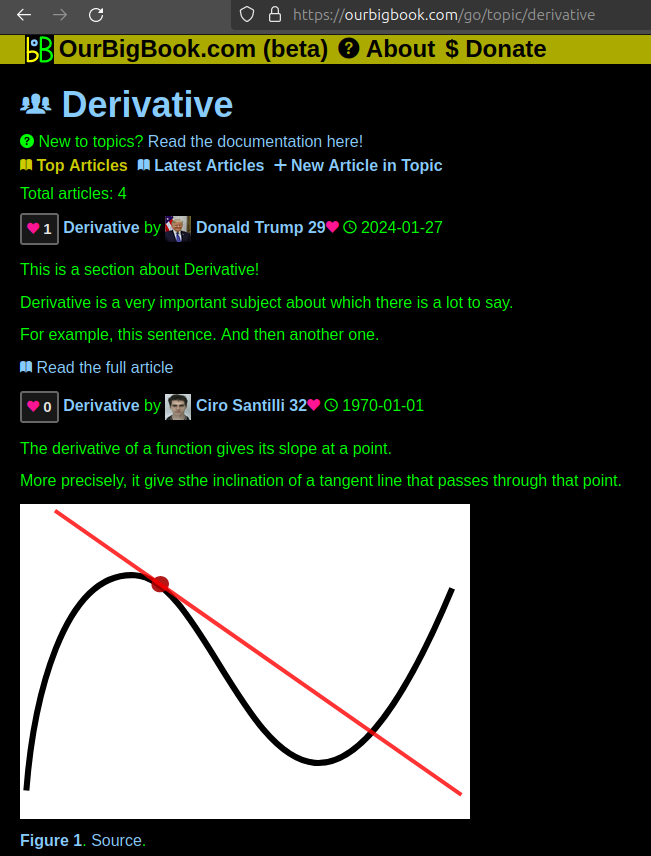
Figure 1. Screenshot of the "Derivative" topic page. View it live at: ourbigbook.com/go/topic/derivativeVideo 2. OurBigBook Web topics demo. Source. - local editing: you can store all your personal knowledge base content locally in a plaintext markup format that can be edited locally and published either:This way you can be sure that even if OurBigBook.com were to go down one day (which we have no plans to do as it is quite cheap to host!), your content will still be perfectly readable as a static site.
- to OurBigBook.com to get awesome multi-user features like topics and likes
- as HTML files to a static website, which you can host yourself for free on many external providers like GitHub Pages, and remain in full control

Figure 3. Visual Studio Code extension installation.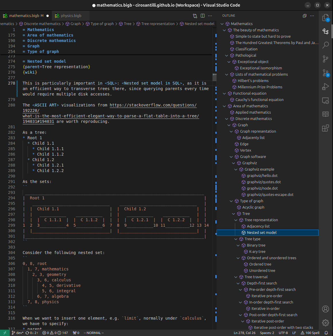
Figure 4. Visual Studio Code extension tree navigation.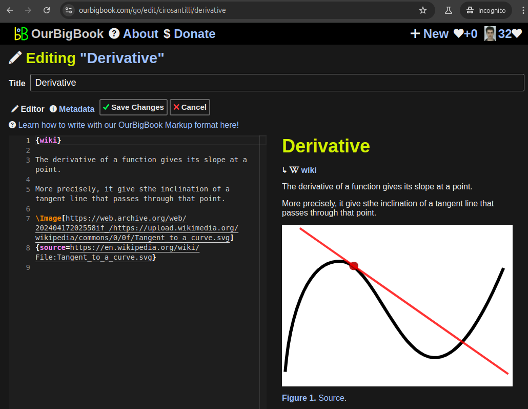
Figure 5. Web editor. You can also edit articles on the Web editor without installing anything locally.Video 3. Edit locally and publish demo. Source. This shows editing OurBigBook Markup and publishing it using the Visual Studio Code extension.Video 4. OurBigBook Visual Studio Code extension editing and navigation demo. Source. 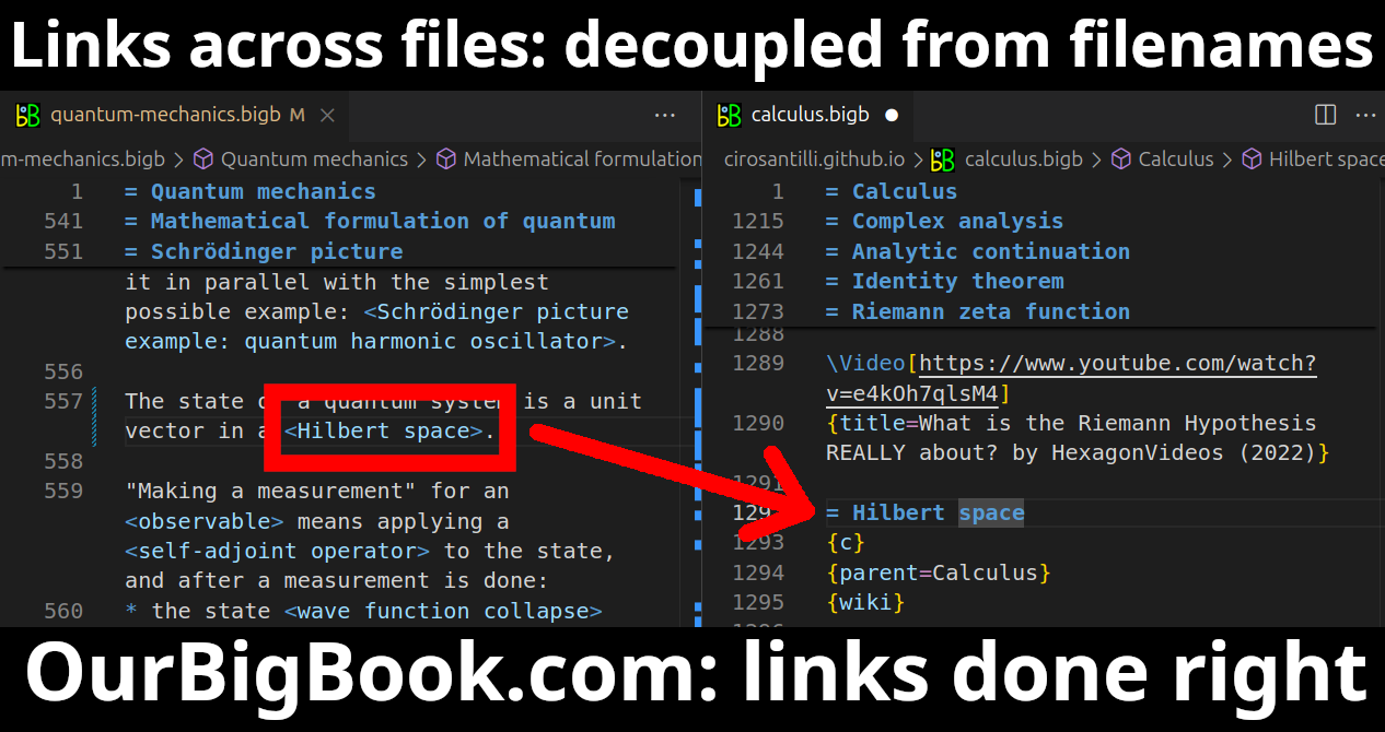
- Infinitely deep tables of contents:

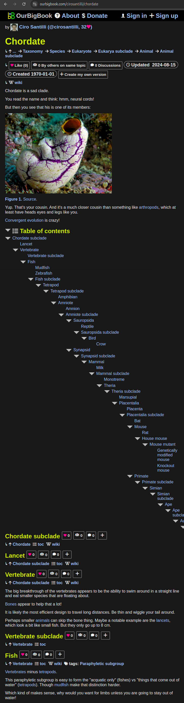
All our software is open source and hosted at: github.com/ourbigbook/ourbigbook
Further documentation can be found at: docs.ourbigbook.com
Feel free to reach our to us for any help or suggestions: docs.ourbigbook.com/#contact