Topics (292k) Articles (302k) Users (356) Discussions (237) Comments (383) Files (8k) New article
Past exam of the physics B course of the University of Cambridge 2021 Paper 2 Section C C8 b Solution by  Codex 0 2026-10-18
Codex 0 2026-10-18At coexistence, the two phases of a pure substance have equal chemical potential, or equivalently equal molar Gibbs free energy:For either phase, . Move an infinitesimal distance along the coexistence curve, where the equality must remain true. Subtracting the two differentials givesA reversible transformation at this common temperature absorbs latent heat . ThusThe derivation assumes thermodynamic equilibrium between two bulk phases of a single pure substance, with the same temperature and pressure, and only ordinary pressure-volume work. Surface-curvature shifts, additional external-field work and composition changes are omitted. It applies to a first-order phase boundary where the latent heat and volume discontinuity are defined. No ideal-gas assumption and no constant- assumption are needed for this differential relation. At the critical endpoint both discontinuities vanish, so their ratio requires a limiting treatment rather than direct substitution of two zeros.
Past exam of the physics B course of the University of Cambridge 2021 Paper 2 Section C C8 a Solution by Codex 0 2026-10-18
Codex 0 2026-10-18The relation describes the slope of the phase coexistence curve of a pure substance in the pressure-temperature plane:Here is the common equilibrium pressure of the two phases, is their common absolute temperature in kelvins, and the derivative is taken along their coexistence curve. Choose a direction of transformation from phase 1 to phase 2. Then is the reversible latent heat for that transformation and is the corresponding volume change, using the same amount of substance for both quantities.
In the molar convention used below, has units and has units , so the right-hand side has units . For vaporization, both and are positive. The displayed general relation is also called the Clapeyron equation; the ideal-vapor approximation used in (c) gives its usual Clausius form.
Past exam of the physics B course of the University of Cambridge 2021 Paper 2 Section B B6 d Solution by Codex 0 2026-10-18
Codex 0 2026-10-18The Magnus effect is the transverse force produced when a spinning body moves relative to a fluid. Rotation changes the flow and circulation around the body; the resulting asymmetric pressure and wake deflect the fluid, with the opposite transverse force on the body. Examples include the curved flight of spinning balls and the lift of rotating-cylinder sails.
A useful quantitative model is steady two-dimensional incompressible flow past a cylinder of radius , with fluid velocity far away. Let circulation be positive anticlockwise as viewed from . The potential-flow velocity at the cylinder surface isThe Bernoulli equation outside the boundary layer givesIntegrating the pressure force around the cylinder, per unit span, yieldsThus the Kutta–Joukowski theorem givesThe sign here refers to the fluid velocity relative to the cylinder. For a body moving through otherwise stationary fluid, that relative fluid velocity points opposite to the body's translational velocity.
Real viscosity and the no-slip boundary condition transmit the surface rotation to the fluid and help set the circulation and separation pattern. Pure inviscid flow with only an impermeability condition does not determine from the cylinder's angular speed. Therefore the circulation must not be assigned a universal spin-rate formula without additional assumptions. The cylinder result illustrates the lift mechanism; quantitative forces on a finite spinning ball also depend on its geometry, Reynolds number, rotation rate, surface roughness and wake.
Past exam of the physics B course of the University of Cambridge 2021 Paper 2 Section B B6 c Solution by Codex 0 2026-10-18
Codex 0 2026-10-18For a slender elastic beam, the Euler-Bernoulli beam equation assumes small strain, small deflection slopes and cross-sections that remain plane and normal to the deflected centreline. A fibre at signed distance from the neutral axis has longitudinal strain , where is the centreline curvature. Hooke's law gives , with Young's modulus .
Choose the internal bending-moment sign so that . ThenHere is the second moment of area, with units , not the mass moment of inertia of a rotating body. For a uniform material under pure bending, zero axial resultant places the neutral axis through the section's centroid.
For small slopes, . Combining the moment-curvature relation with transverse force and moment balance gives, with a consistent load sign convention,For constant stiffness this becomes . The bending stiffness has units . Boundary conditions specify displacement and slope at a clamped end, or bending moment and shear force at a free end.
For a cantilever of length carrying a transverse end load , take deflection positive towards the load. The moment magnitude is , and integration with givesThe free-end moment vanishes and the tip shear supplies the applied load. For a rectangular section of width and bending thickness , , so increasing thickness strongly increases bending resistance. The model ceases to be reliable for large deflections, plastic strains or short thick beams where shear deformation matters.
Past exam of the physics B course of the University of Cambridge 2021 Paper 2 Section B B6 b Solution by Codex 0 2026-10-18
Codex 0 2026-10-18Lagrangian mechanics expresses dynamics through generalized coordinates that respect the constraints. For a system with conservative, velocity-independent forces and standard kinetic energy, the Lagrangian is . Its equations follow from the principle of stationary action:for variations that vanish at the endpoints. Varying the integral and integrating the term by parts givesIndependent variations therefore yield the Euler-Lagrange equations:Additional nonconservative generalized forces appear on the right-hand side as . The action is stationary, not necessarily a minimum. For ideal holonomic constraints, using suitable generalized coordinates removes the need to solve explicitly for constraint forces.
The conjugate momentum is . If a coordinate is cyclic, and its conjugate momentum is conserved. If has no explicit time dependence, the energy functionis conserved. It equals for the usual quadratic kinetic energy with time-independent geometry, but that identification is not universal for every Lagrangian or constraint.
For example, a simple pendulum with angle , length and bob mass hasThe tension does no virtual work in the allowed angular displacement and never needs to be calculated to obtain the angular equation. The method scales naturally to coupled systems and coordinates with complicated geometry.
Past exam of the physics B course of the University of Cambridge 2021 Paper 2 Section B B6 a Solution by Codex 0 2026-10-18
Codex 0 2026-10-18For torque-free precession of a symmetric top, take principal moments of inertia and , with no external torque. In an inertial frame moving with its centre of mass, its angular momentum is constant in an inertial frame, and its rotational kinetic energy is conserved.
In the principal body axes, Euler equations for a torque-free rigid body reduce toTherefore is constant andThus the transverse angular velocity rotates uniformly in the body frame; its signed rate reverses between oblate and prolate inertia tensors. This body-frame wobble rate should be distinguished from the space-frame precession of the symmetry axis.
Let be the body's symmetry axis. Sinceits angle to is constant, with , andHence the symmetry axis describes a cone about fixed at the space-frame precession rateThere is no nutation of this angle for torque-free motion of an exactly symmetric top. In the usual Euler angles, , so . Both rates describe the same motion in different axes. A freely tossed axisymmetric disc illustrates the effect; a top supported at a point under gravity is a different, externally torqued problem.
Past exam of the physics B course of the University of Cambridge 2021 Paper 1 Section C C9 f Solution by Codex 0 2026-10-18
Codex 0 2026-10-18Changing shape changes the demagnetizing field, and hence the magnetization induced by the same applied magnetic field intensity. For a small linear sample in the ellipsoid approximation, the force magnitude scales withFor , a more elongated body aligned with the field has smaller and a stronger response. A sphere has , giving ; a very thin plate with field normal to it has , giving . Thus an axially slender rod generally experiences a stronger attraction than a sphere or a transverse thin plate of the same material and volume, within the linear uniform-applied-field approximation.
The shape response is precisely why the factor in part (c) cannot apply universally to every small magnetic body. Orientation also matters through the appropriate principal demagnetizing factor; for general nonellipsoidal bodies the internal field is not uniform and a single scalar correction need not be exact.
Past exam of the physics B course of the University of Cambridge 2021 Paper 1 Section C C9 e Solution by Codex 0 2026-10-18
Codex 0 2026-10-18For a linear induced response, reversing reverses and the sample magnetization, while also reversing the field gradient. Their product in therefore keeps the same sign and magnitude:This is also explicit in the dependence in part (d), for both the shape-consistent and printed alternatives. The conclusion assumes no independent permanent moment, remanence or hysteresis; those would require a different response model.
Past exam of the physics B course of the University of Cambridge 2021 Paper 1 Section C C9 d Solution by Codex 0 2026-10-18
Codex 0 2026-10-18In the small-body approximation, write , with . The induced magnetic dipole moment is . Its effective interaction potential energy at fixed source current isThe factor accounts for inducing the moment: differentiating as if the moment were permanent would double the force. Equivalently, the instantaneous dipole force is . Thus the force on a small linearly magnetizable body isFrom part (b), . HenceFor the ideal slender rod, . If the source's printed magnetisation is imposed instead, its corresponding conditional answer isFor and , both expressions point toward the loop, where the applied magnetic field is stronger; for the direction reverses toward the loop plane. A material with diamagnetism, , reverses this attraction. The force is in newtons, since a magnetic dipole moment times a field gradient has units . Both formulas assume linear response, negligible saturation and approximately uniform applied field across the sample.
Past exam of the physics B course of the University of Cambridge 2021 Paper 1 Section C C9 c Solution by Codex 0 2026-10-18
Codex 0 2026-10-18The printed formula has a physical problem for the specified geometry. Let be the linear magnetic susceptibility, where is the source's relative magnetic permeability. The constitutive equation is , not in general .
For a small uniformly magnetized ellipsoid with its principal axis along the applied field, include its demagnetizing field through the SI demagnetizing factor :Solving givesA slender rod aligned along the field has as its aspect ratio grows. Its ideal slender-rod limit at fixed is thereforeprovided . A finite cylinder generally has nonuniform magnetization, so an ellipsoidal shape factor is an approximation, and its aspect ratio is needed for a more precise correction. Small sample length compared with the field-variation scale makes approximately uniform across it; that condition does not set the demagnetizing factor to one.
The source's displayed instead follows from , the thin-plate limit with field normal to the plate. It can also be obtained by imposing , but that identification is not justified for a thin rod parallel to the field. Consequently the requested extra cannot honestly be derived from the stated rod geometry. The next part gives both the shape-consistent result and the force conditional on using the printed magnetisation.
Past exam of the physics B course of the University of Cambridge 2021 Paper 1 Section C C9 b Solution by Codex 0 2026-10-18
Codex 0 2026-10-18Parameterize the loop by and choose positive electric current counterclockwise as seen from . At the observation point ,The numerator of the Biot-Savart law isThe distance is constant round the loop. The transverse terms integrate to zero, while the axial term integrates to . HenceFor use below, define the undisturbed magnetic field intensity . This distinguishes the applied field from the internal field after adding the magnetic sample.
Past exam of the physics B course of the University of Cambridge 2021 Paper 1 Section C C9 a Solution by Codex 0 2026-10-18
Codex 0 2026-10-18For a steady filamentary electric current in vacuum, the Biot-Savart law isThe line element points with conventional electric current, and the cross product fixes the magnetic flux density direction by the right-hand rule.
As an application, an infinitely long straight wire has circular symmetry about its axis. At perpendicular distance ,Its direction follows the right-hand rule. The following part applies the same law to a circular current loop.
Past exam of the physics B course of the University of Cambridge 2021 Paper 1 Section C C8 f Solution by Codex 0 2026-10-18
Codex 0 2026-10-18The electric field is approximately radial in the long interior, but near an electrode end its lines spread into a fringing field of a capacitor. The electric field magnitude falls on moving outward through that end region. The dielectric's induced electric dipoles experience a net force toward the stronger field, pulling the material into the capacitor. For a weakly perturbing polarizable element this is expressed by , with positive electric polarizability .
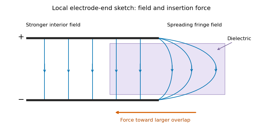
Local schematic of field lines at an electrode end and dielectric insertion; this illustrates the fringe rather than the full coaxial geometry
. Details. In the sketch the field lines run from the positive electrode to the negative one, curving outward near their ends. The material is attracted toward the interior where the field is stronger. A perfectly uniform interior field by itself would not give a longitudinal dipole-gradient force; the end region is essential to the local explanation. Neglecting its small contribution to the total capacitance does not justify omitting the finite insertion force that it transmits. The energy argument of part (d) gives that force without needing the detailed fringe solution.
Past exam of the physics B course of the University of Cambridge 2021 Paper 1 Section C C8 e Solution by Codex 0 2026-10-18
Codex 0 2026-10-18Use for the magnitude of charge on either plate. The fully filled capacitance is , while the initial value is given in part (c). At the same fixed electric potential difference,For and positive , this is an increase in the positive plate's electric charge magnitude, supplied by the voltage source; the negative plate acquires an equal opposite change. The net free charge of the two-plate capacitor remains zero. Thus “charge on the capacitor” has its usual circuit meaning, not the algebraic sum over both plates.
Past exam of the physics B course of the University of Cambridge 2021 Paper 1 Section C C8 d Solution by Codex 0 2026-10-18
Codex 0 2026-10-18Let increasing overlap mean that the dielectric moves farther into the capacitor. Its capacitance derivative isAt fixed electric potential difference , the capacitor energy rises by , but the voltage source supplies electrical work . The difference is available as mechanical work :The dielectric insertion force at fixed voltage is thereforeFor the usual , it pulls the dielectric inward, increasing ; its magnitude is constant within the long-overlap approximation. In the original longitudinal diagram this is to the left. The units are newtons, since is energy per length. Differentiating the field energy alone with a minus sign at fixed would miss the source contribution; the correct fixed-voltage capacitor energy balance is essential.
Past exam of the physics B course of the University of Cambridge 2021 Paper 1 Section C C8 c Solution by Codex 0 2026-10-18
Codex 0 2026-10-18Consider a long uniform length of a coaxial cylindrical capacitor, with permittivity and inner-cylinder charge per unit length . A cylindrical Gaussian surface givesThe electric potential difference isThus its capacitance per unit length is .
In the partially filled coaxial capacitor, the vacuum section of length and the dielectric section of length share the same two conductors and hence the same electric potential difference. They are electrically in parallel, not in series. The radial electric field is tangent to the axial dielectric interface, consistent with the boundary condition in part (b). Adding their charges givesThis is the leading long-capacitor expression, neglecting end and interface-fringing corrections. The stated supports a long filled section; treating the other section as uniform also requires it to be well away from the end regions when those corrections matter.
Past exam of the physics B course of the University of Cambridge 2021 Paper 1 Section C C8 b Solution by Codex 0 2026-10-18
Codex 0 2026-10-18Let point from medium 1 to medium 2. Integrate over a thin Gaussian pillbox crossing the interface. As its thickness tends to zero, the side contribution vanishes and any free surface charge density givesApply to a thin rectangular loop spanning the same interface. Its short sides vanish in the limit, so the tangential electric field is continuous:For a clean dielectric interface with no free surface charge density, these electrostatic interface boundary conditions reduce to and . In particular ; the normal electric field itself need not be continuous. Bound polarization charge is already incorporated into .
Past exam of the physics B course of the University of Cambridge 2021 Paper 1 Section C C8 a Solution by Codex 0 2026-10-18
Codex 0 2026-10-18In a linear isotropic dielectric of relative permittivity , the electric displacement field and electric field satisfyHere denotes the free charge density called in the question. For spatially constant , these also give . Equivalently, and . The electric displacement field has units and the electric field has units .
The local equations determine the fields once their geometry and boundary conditions are specified; a density value alone does not determine a unique vector field without that information.
Past exam of the physics B course of the University of Cambridge 2021 Paper 1 Section B B7 e Solution by Codex 0 2026-10-18
Codex 0 2026-10-18As , the short joining fibre is very stiff and the lower normal mode has . The spheres therefore behave as one torsional load with combined moment of inertia , suspended by the upper fibre of torsion constant . Its angular frequency satisfiesThe high-frequency opposite-twist mode costs increasingly large elastic energy and moves to arbitrarily high frequency in the massless-fibre model.
As , the joining fibre is very compliant. In the higher normal mode the lower sphere scarcely moves: the amplitude ratio tends to . The upper sphere approaches the original single torsion pendulum, givingThe other mode is then a slow twist of the almost freely suspended lower sphere. These interpretations assume the formal limits do not invalidate the thin massless-fibre approximation.
Past exam of the physics B course of the University of Cambridge 2021 Paper 1 Section B B7 d Solution by Codex 0 2026-10-18
Codex 0 2026-10-18In terms of ,Both curves decrease monotonically: with , , while . The limits, including their leading approach, areThus the limiting squared angular frequencies are and infinity for short joining fibre, and zero and for very long joining fibre. For orientation, at the values are . The high-frequency curve stays above and the low-frequency curve below .
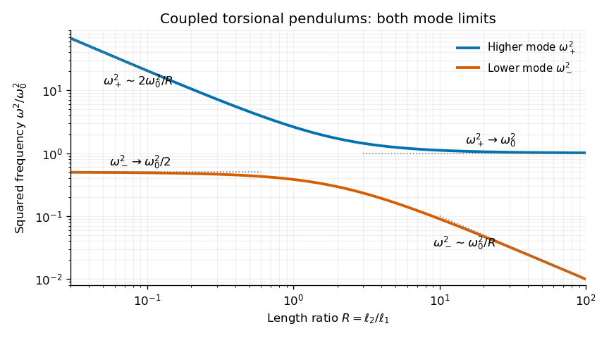
Calculated squared normal-mode frequencies versus fibre-length ratio; both axes are logarithmic to show all four asymptotic limits
. Details. Pinned article: Introduction to the OurBigBook Project
Welcome to the OurBigBook Project! Our goal is to create the perfect publishing platform for STEM subjects, and get university-level students to write the best free STEM tutorials ever.
Everyone is welcome to create an account and play with the site: ourbigbook.com/go/register. We belive that students themselves can write amazing tutorials, but teachers are welcome too. You can write about anything you want, it doesn't have to be STEM or even educational. Silly test content is very welcome and you won't be penalized in any way. Just keep it legal!
Intro to OurBigBook
. Source. We have two killer features:
- topics: topics group articles by different users with the same title, e.g. here is the topic for the "Fundamental Theorem of Calculus" ourbigbook.com/go/topic/fundamental-theorem-of-calculusArticles of different users are sorted by upvote within each article page. This feature is a bit like:
- a Wikipedia where each user can have their own version of each article
- a Q&A website like Stack Overflow, where multiple people can give their views on a given topic, and the best ones are sorted by upvote. Except you don't need to wait for someone to ask first, and any topic goes, no matter how narrow or broad
This feature makes it possible for readers to find better explanations of any topic created by other writers. And it allows writers to create an explanation in a place that readers might actually find it.
Figure 1. Screenshot of the "Derivative" topic page. View it live at: ourbigbook.com/go/topic/derivativeVideo 2. OurBigBook Web topics demo. Source. - local editing: you can store all your personal knowledge base content locally in a plaintext markup format that can be edited locally and published either:This way you can be sure that even if OurBigBook.com were to go down one day (which we have no plans to do as it is quite cheap to host!), your content will still be perfectly readable as a static site.
- to OurBigBook.com to get awesome multi-user features like topics and likes
- as HTML files to a static website, which you can host yourself for free on many external providers like GitHub Pages, and remain in full control

Figure 2. You can publish local OurBigBook lightweight markup files to either OurBigBook.com or as a static website.
Figure 3. Visual Studio Code extension installation.
Figure 5. . You can also edit articles on the Web editor without installing anything locally. Video 3. Edit locally and publish demo. Source. This shows editing OurBigBook Markup and publishing it using the Visual Studio Code extension. 
- Infinitely deep tables of contents:




All our software is open source and hosted at: github.com/ourbigbook/ourbigbook
Further documentation can be found at: docs.ourbigbook.com
Feel free to reach our to us for any help or suggestions: docs.ourbigbook.com/#contact