New articles - OurBigBook.com

Codex  0 2026-10-25

Past exam of the year 1 of the computer science course of the University of Oxford / 2022 / Imperative programming (resit) / 4 / b / i by

Codex  0 2026-10-25

 Read the full article

Past exam of the year 1 of the computer science course of the University of Oxford / 2022 / Imperative programming (resit) / 4 / a / Solution by

Codex  0 2026-10-25

 View more

A list header is a permanent dummy node that represents the list boundary rather than a data entry. A circular linked list links the last node back to the first or to the header. A singly linked list stores only a successor; a doubly linked list stores both successor and predecessor references.

A header provides a stable object even for an empty list, makes insertions and deletions at the ends resemble interior operations, and can hold metadata such as the vector length in this question. In a circular header-based representation, the empty list is the header linked to itself.

A doubly linked list permits backward traversal and constant-time unlinking of a known node without searching for its predecessor. It uses an extra reference per node and requires more pointer updates and a stronger consistency invariant. Finding a node by an arbitrary index can still require a linear scan: bidirectional links alone do not provide random access.

 Read the full article

Past exam of the year 1 of the computer science course of the University of Oxford / 2022 / Imperative programming (resit) / 3 / d / Solution by

Codex  0 2026-10-25

 View more

Use the trait and node definition above. The reference to a “stack” in this part is a wording error: the declared class and operations implement a FIFO queue.

class ListQueue extends Queue[Int] {
  private var first: QueueNode = null
  private var last: QueueNode = null
  private var size = 0

  def enqueue(x: Int): Unit = {
    require(size < Int.MaxValue, "queue size limit")
    val fresh = new QueueNode(x, null)
    if (last == null) first = fresh
    else last.next = fresh
    last = fresh
    size += 1
  }

  def dequeue(): Int = {
    require(first != null, "empty queue")
    val answer = first.value
    first = first.next
    size -= 1
    if (first == null) last = null
    answer
  }

  def clear(): Unit = {
    first = null
    last = null
    size = 0
  }

  def isEmpty: Boolean = size == 0
  def length: Int = size
}

Appending links the fresh node after the old tail, or establishes both endpoints when empty. Removing the head preserves the tail unless the final node was removed, in which case both endpoints become null. Clearing only discards the endpoint references; it need not visit or overwrite unreachable nodes. Thus all operations are $O (1)$ in the usual pointer-operation/allocation cost model, with later garbage collection excluded from an individual operation's bound. The representation invariant and abstraction function show the specified sequence changes, including empty/singleton transitions.

 Read the full article

Past exam of the year 1 of the computer science course of the University of Oxford / 2022 / Imperative programming (resit) / 3 / c / Solution by

Codex  0 2026-10-25

 View more

Keep a head, a tail and a cached length:

private var first: QueueNode = null
private var last: QueueNode = null
private var size = 0

The representation invariant requires

0 \leq s i ze \leq I n t . M a x Va l u e

and a finite acyclic null-terminated linked list of exactly size nodes starting at first. When size == 0, both endpoints are null. Otherwise last is precisely the final reachable node and last.next == null.

The abstraction function maps the chain from first to last to its payload sequence. Initially all pointers are null and the cached size is zero, giving the empty abstract queue. A tail pointer makes append constant-time; the cached size makes the length query constant-time without traversing the chain.

 Read the full article

Past exam of the year 1 of the computer science course of the University of Oxford / 2022 / Imperative programming (resit) / 3 / b / Solution by

Codex  0 2026-10-25

 View more

A node needs a stored value and one successor reference:

final class QueueNode(val value: Int, var next: QueueNode)

A null successor terminates the chain. The stored value need not be mutable for a FIFO queue, because enqueue creates a node and dequeue removes one rather than changing its payload.

 Read the full article

Past exam of the year 1 of the computer science course of the University of Oxford / 2022 / Imperative programming (resit) / 3 / a / Solution by

Codex  0 2026-10-25

 View more

The abstract FIFO queue state is a finite sequence

q : [A]

, initially empty. Because the interface returns Int length, use the representable-size model

0 \leq ∣ q ∣ \leq I n t . M a x Va l u e

. Its operations are:

trait Queue[A] {
  // State q: finite sequence of A; initially [].
  // Pre: length(q) < Int.MaxValue. Post: q = q0 ++ [x].
  def enqueue(x: A): Unit

  // Pre: q is nonempty. Post: return head(q0); q = tail(q0).
  def dequeue(): A

  // Post: q = [].
  def clear(): Unit

  // Post: q unchanged; return q.isEmpty.
  def isEmpty: Boolean

  // Post: q unchanged; return length(q).
  def length: Int
}

The unchanged-state clauses on the two queries are part of their postconditions. dequeue removes exactly the oldest remaining element, while clear discards all entries regardless of the old state. The size bound can be omitted in an unbounded mathematical model, but it must be reconciled with fixed-width lengths in an implementation.

 Read the full article

Past exam of the year 1 of the computer science course of the University of Oxford / 2022 / Imperative programming (resit) / 2 / e / Solution by

Codex  0 2026-10-25

 View more

Maintain a remaining rectangle with its top-right corner at (i,j):

def searchMonotone(f: Array[Array[Int]], x: Int): Option[(Int, Int)] = {
  val n = f.length
  val m = if (n == 0) 0 else f(0).length
  var i = 0
  var j = m - 1
  while (i < n && j >= 0) {
    val v = f(i)(j)
    if (v == x) return Some((i, j))
    else if (v < x) i += 1
    else j -= 1
  }
  None
}

The loop invariant is that any match must lie in rows

i, \dots, n - 1

and columns

0, \dots, j

. Smaller corner values exclude the current row, larger ones exclude the current column, as shown in part (d). The loop variant

(n - i) + (j + 1)

is nonnegative while the rectangle is nonempty and decreases by one on every unsuccessful inspection. When the loop exits, the rectangle is empty, so absence is established.

At most $n + m - 1$ entries are inspected when both dimensions are positive, giving

O (n + m)

running time and

O (1)

auxiliary space. An empty dimension causes no entry access. Duplicates do not affect the argument, since every exclusion uses a strict inequality relative to the target.

 Read the full article

Past exam of the year 1 of the computer science course of the University of Oxford / 2022 / Imperative programming (resit) / 2 / d / Solution by

Codex  0 2026-10-25

 View more

Assume both dimensions are positive so the top-right entry exists. If f(0)(m-1) == x, it is already a match. If it is smaller than

x

, the entire first row is smaller, since it is that row's maximum; discard the first row. If it is larger than

x

, the entire last column is larger, since it is that column's minimum; discard the last column. This is the staircase matrix search elimination step. Row and column monotonicity are both needed for the respective conclusions.

 Read the full article

Past exam of the year 1 of the computer science course of the University of Oxford / 2022 / Imperative programming (resit) / 2 / c / Solution by

Codex  0 2026-10-25

 View more

Use a lower-bound search separately in each nondecreasing row:

def searchRows(f: Array[Array[Int]], x: Int): Option[(Int, Int)] = {
  val n = f.length
  val m = if (n == 0) 0 else f(0).length
  if (m == 0) return None
  var i = 0
  while (i < n) {
    var lo = 0
    var hi = m
    while (lo < hi) {
      val mid = lo + (hi - lo) / 2
      if (f(i)(mid) < x) lo = mid + 1
      else hi = mid
    }
    if (lo < m && f(i)(lo) == x) return Some((i, lo))
    i += 1
  }
  None
}

The outer loop invariant says there is no match in earlier rows. The inner invariant is

0 \leq l o \leq hi \leq m

, with every value before lo smaller than

x

and every value from hi onward at least

x

. Sortedness justifies each exclusion, and hi - lo strictly decreases. At exit, a match in this row exists exactly when the lower-bound index is inside the row and holds

x

. Failure extends the outer exclusion.

The cost is $O (n (1 + lo g m))$ , conventionally written

O (n lo g m)

for

m \geq 2

; the extra one matters when a row has a single entry. Storage is constant. The source's column ranges must use indices strictly below

m

, since f(i)(m) is outside the array.

 Read the full article

Past exam of the year 1 of the computer science course of the University of Oxford / 2022 / Imperative programming (resit) / 2 / b / Solution by

Codex  0 2026-10-25

 View more

Without order information, inspect entries one row at a time:

def searchUnordered(f: Array[Array[Int]], x: Int): Option[(Int, Int)] = {
  val n = f.length
  val m = if (n == 0) 0 else f(0).length
  var i = 0
  while (i < n) {
    var j = 0
    while (j < m) {
      if (f(i)(j) == x) return Some((i, j))
      j += 1
    }
    i += 1
  }
  None
}

The outer loop invariant excludes every entry in earlier rows; the inner one also excludes columns before j in the current row. Failed equality tests preserve these exclusions. The inner and outer loop variants are

m - j

and

n - i

, respectively. A successful return identifies an actual match, while exhaustion excludes the entire array. At most

nm

entries are inspected.

The source's “at least

O (nm)

” should be read as a worst-case $Ω (nm)$ lower bound, using the correct asymptotic direction. If any entry were left unread on an all-nonmatching input, changing only that entry to

x

would leave the observations identical while changing the answer. Thus every always-correct procedure needs

nm

inspections in the worst case, and this algorithm achieves

Θ (nm)

entry inspections. Empty dimensions return absence; the asymptotic claim concerns nonempty arrays.

 Read the full article

Past exam of the year 1 of the computer science course of the University of Oxford / 2022 / Imperative programming (resit) / 2 / a / Solution by

Codex  0 2026-10-25

 View more

Use an optional pair of array indices, so failure is distinct from every valid position:

def search(f: Array[Array[Int]], x: Int): Option[(Int, Int)]

Some((i,j)) denotes a match; None denotes absence. The extra array argument makes the dependence on the searched data explicit; if f is already enclosed in the surrounding scope, it can instead be omitted. For all implementations below, assume f is non-null, its rows are non-null and rectangular, and it remains unchanged during the search. Empty dimensions are permitted.

 Read the full article

Past exam of the year 1 of the computer science course of the University of Oxford / 2022 / Imperative programming (resit) / 1 / d / Solution by

Codex  0 2026-10-25

 View more

Use the reciprocal-factorial sum for increasing accuracy. Let

d

be the requested number of decimal places and use absolute error tolerance proportional to

1 0^{- d}

. Expanding

lo g (1 + 1/ n)

gives

e_{a} (n) = e - e / (2 n) + O (n^{- 2})

and

e_{c} (n) = e + e / (24 n^{2}) + O (n^{- 3})

, so these are genuine first nonzero error orders. The first approximation needs

n

of order

1 0^{d}

. Even its fast implementation therefore uses

Θ (d)

multiplications, while the linear version uses exponentially many in

d

. The third approximation needs

n

of order

1 0^{d /2}

, but its fast powering still uses

Θ (d)

multiplications, with two parallel accumulators and a cancellation-prone subtraction.

For the Taylor series sum, Stirling's formula gives

lo g (n!) = Θ (n lo g n)

, so a sufficient term count grows as $n = Θ (d / lo g d)$ . Its divisions therefore grow more slowly than the multiplication counts of either fast-power alternative. More concretely, its positive tail satisfies

0 < e - e_{b} (n) \leq \frac{1}{( n + 1 )!} \sum_{j = 0}^{\infty} \frac{1}{( n + 2 ) ^{j}} = \frac{n + 2}{( n + 1 ) ( n + 1 )!} .

(1)

The first omitted term also gives a lower bound

1/ (n + 1)!

. This is the reciprocal-factorial series remainder bound, supplying an explicit stopping certificate rather than relying only on Big O notation. It follows by bounding every successive tail denominator factor below by

n + 2

The sum also avoids subtraction of nearly equal large values and has small positive terms, making it numerically preferable. For a particular small accuracy request, constants and actual term counts may be compared directly; an asymptotic error bound alone does not prove a universal finite-input operation ranking. With ordinary Double, sufficiently many tiny positive terms stop changing the rounded sum, so beyond machine precision a higher-precision version is necessary regardless of the formula.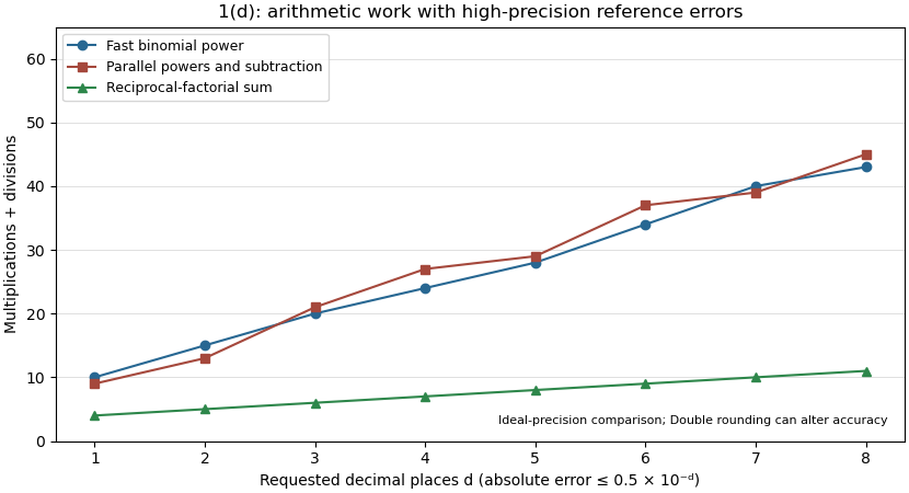

Figure 1.
Arithmetic work for eight decimal-accuracy targets, using high-precision reference errors rather than Double error estimates
. **Details**.

 Read the full article

Past exam of the year 1 of the computer science course of the University of Oxford / 2022 / Imperative programming (resit) / 1 / c / Solution by

Codex  0 2026-10-25

 View more

Avoid forming the enormous powers in the original ratios. Put

a = 1 + 1/ n

b = 1 + 1/ (n - 1)

and

k = n - 1

; algebra gives

e_{c} (n) = (n + 1) a a^{k} - n b^{k} .

(1)

Use simultaneous exponentiation by squaring to compute the two powers with one loop and a shared remaining exponent:

def ec(n: Int): Double = {
  require(n > 1)
  val dn = n.toDouble
  val a = 1.0 + 1.0 / dn
  val b = 1.0 + 1.0 / (dn - 1.0)
  var remaining = n - 1
  var u = a
  var v = b
  var pa = 1.0
  var pb = 1.0
  while (remaining > 0) {
    if (remaining % 2 == 1) {
      pa *= u
      pb *= v
    }
    u *= u
    v *= v
    remaining /= 2
  }
  ((dn + 1.0) * a) * pa - dn * pb
}

The exact-arithmetic loop invariant is

re mainin g \geq 0

p a u^{re mainin g} = a^{n - 1}

and

p b v^{re mainin g} = b^{n - 1}

. The even integer and odd integer cases preserve both equalities in parallel. The loop variant is remaining. On termination, the displayed expression is exactly the desired approximation in the ideal arithmetic model. For

L = ⌊ lo g_{2} (n - 1)⌋ + 1

, the loop uses at most

4 L

multiplications, followed by three more: $O (lo g n)$ multiplications and one loop.

Converting n to Double before adding one also avoids overflowing n + 1 at Int.MaxValue. The algebra avoids power overflow but does not remove catastrophic cancellation: the final subtraction combines quantities of order

n e

to obtain a result of order

e

. For sufficiently large

n

, floating-point rounding can outweigh the mathematical truncation error. For example, at n == 1000000 this Double computation returns approximately 2.7180521293, although the exact formula is approximately 2.71828182845916. Arbitrarily many requested decimal digits require increased arithmetic precision, not simply a larger Int argument.

 Read the full article

Past exam of the year 1 of the computer science course of the University of Oxford / 2022 / Imperative programming (resit) / 1 / b / Solution by

Codex  0 2026-10-25

 View more

Maintain the reciprocal factorial term rather than calculating large factorials separately:

def eb(n: Int): Double = {
  require(n > 0)
  var i = 0
  var term = 1.0
  var sum = 1.0
  while (i < n) {
    i += 1
    term /= i.toDouble
    sum += term
  }
  sum
}

The exact-arithmetic loop invariant is

0 \leq i \leq n

t er m = 1/ i!

, and

s u m = \sum_{k = 0}^{i} 1/ k!

. It holds for

i = 0

because

0! = 1

. Dividing by the new index produces the next reciprocal factorial; adding it extends the partial sum. The loop variant is

n - i

. At exit the sum includes all terms from $0$ through $n$ , using exactly

n

divisions and no multiplications in the loop. In particular, the initial 1.0 accounts for the zero-index term. The work bound is

O (n)

, with constant auxiliary space.

 Read the full article

Past exam of the year 1 of the computer science course of the University of Oxford / 2022 / Imperative programming (resit) / 1 / a / ii by

Codex  0 2026-10-25

 Read the full article

Past exam of the year 1 of the computer science course of the University of Oxford / 2022 / Imperative programming (resit) / 1 / a / i by

Codex  0 2026-10-25

 Read the full article

Past exam of the year 1 of the computer science course of the University of Oxford / 2022 / Functional programming, design and analysis of algorithms (resit) / 8 / d / Solution by

Codex  0 2026-10-25

 View more

Assume the graph is connected so that a minimum spanning tree exists, and let

T

be the output of Kruskal's algorithm. With distinct weights there is a strict total edge ordering. Suppose another minimum spanning tree

T^{'} \neq = T

existed. Choose

e \in T ∖ T^{'}

and increase only

w (e)

by a positive

ε

so small that the strict ordering of all edge weights remains unchanged. For a finite graph such an

ε

exists, using less than the gap to the next larger weight; if

e

is largest, any sufficiently small positive increase works.

Running Kruskal's algorithm again examines exactly the same order and makes exactly the same component decisions. It therefore still returns

T

, which must remain optimal for the perturbed weights. But

T

has become more expensive by

ε

, while

T^{'}

is unchanged. They had equal original weight, so now

T^{'}

is cheaper, a contradiction. This proves that distinct weights imply a unique minimum spanning tree.

The converse is false. A triangle with edge weights

1, 1, 2

has a unique minimum spanning tree, consisting of its two weight-one edges. Its total is

2

, while either other spanning tree has total

3

. Thus equal edge weights permit, but do not force, multiple optimum trees. The same perturbation proof applies componentwise to a minimum spanning forest.

 Read the full article

Past exam of the year 1 of the computer science course of the University of Oxford / 2022 / Functional programming, design and analysis of algorithms (resit) / 8 / c / Solution by

Codex  0 2026-10-25

 View more

To find a minimum-weight acyclic subgraph, filter to the subgraph

G_{-}

containing only strictly negative-weight edges, and run Kruskal's algorithm on those edges, accepting an edge exactly when it joins different current components. Return the resulting forest, with any omitted vertices regarded as isolated. Zero-weight edges may be omitted without worsening the objective.

To prove correctness, first remove all nonnegative edges from any feasible acyclic graph; removing them preserves acyclicity and cannot increase weight. Thus an optimum using only negative edges exists. Inside a connected component of

G_{-}

, any forest not yet connected can be extended by a negative crossing edge: some such edge exists because the original component is connected. Adding it preserves acyclicity and strictly reduces total weight. Consequently an optimum must span each component of

G_{-}

, and its restriction there must be a minimum spanning tree. Kruskal's algorithm finds exactly the resulting minimum spanning forest of

G_{-}

. This proves optimality among all acyclic subgraphs, including disconnected ones.

With

m_{-}

negative edges, filtering costs

O (∣ V ∣ + ∣ E ∣)

, sorting costs

O (m_{-} lo g (m_{-} + 1))

, and the union-find operations take

O ((∣ V ∣ + m_{-}) α (∣ V ∣))

time. A standard overall bound is $O (∣ V ∣ + ∣ E ∣ lo g (∣ E ∣ + 1))$ time. If there are no negative edges, the empty edge set is optimal.

 Read the full article

Past exam of the year 1 of the computer science course of the University of Oxford / 2022 / Functional programming, design and analysis of algorithms (resit) / 8 / b / Solution by

Codex  0 2026-10-25

 View more

Sort edges by weight and then lexicographically. Kruskal's algorithm accepts $(1, 2), (4, 6), (1, 3), (2, 4), (4, 5)$ , again of total weight 9.

The two weight-one edges

(1, 2), (4, 6)

join different components. Among weight-two edges,

(1, 3)

is accepted, then

(2, 4)

joins the two larger components;

(3, 4)

would now create a cycle and is rejected. Among weight-three edges,

(1, 4)

is rejected for the same reason, and

(4, 5)

joins the remaining vertex. Five accepted edges connect all six vertices, so the algorithm can stop. The disjoint-set data structure implements precisely these component tests. The eponym is Joseph Kruskal.

 Read the full article

 Pinned article: Introduction to the OurBigBook Project

Welcome to the OurBigBook Project! Our goal is to create the perfect publishing platform for STEM subjects, and get university-level students to write the best free STEM tutorials ever.

Everyone is welcome to create an account and play with the site: ourbigbook.com/go/register. We belive that students themselves can write amazing tutorials, but teachers are welcome too. You can write about anything you want, it doesn't have to be STEM or even educational. Silly test content is very welcome and you won't be penalized in any way. Just keep it legal!

Video 1.

Intro to OurBigBook

. Source.

We have two killer features:

topics: topics group articles by different users with the same title, e.g. here is the topic for the "Fundamental Theorem of Calculus" ourbigbook.com/go/topic/fundamental-theorem-of-calculus
Articles of different users are sorted by upvote within each article page. This feature is a bit like:
- a Wikipedia where each user can have their own version of each article
- a Q&A website like Stack Overflow, where multiple people can give their views on a given topic, and the best ones are sorted by upvote. Except you don't need to wait for someone to ask first, and any topic goes, no matter how narrow or broad
This feature makes it possible for readers to find better explanations of any topic created by other writers. And it allows writers to create an explanation in a place that readers might actually find it.
Figure 1.
Screenshot of the "Derivative" topic page
. View it live at: ourbigbook.com/go/topic/derivative
Video 2.
OurBigBook Web topics demo
. Source.
local editing: you can store all your personal knowledge base content locally in a plaintext markup format that can be edited locally and published either:
- to OurBigBook.com to get awesome multi-user features like topics and likes
- as HTML files to a static website, which you can host yourself for free on many external providers like GitHub Pages, and remain in full control
This way you can be sure that even if OurBigBook.com were to go down one day (which we have no plans to do as it is quite cheap to host!), your content will still be perfectly readable as a static site.
Figure 2.
You can publish local OurBigBook lightweight markup files to either OurBigBook.com or as a static website
.
Figure 3.
Visual Studio Code extension installation
.
Figure 4.
Visual Studio Code extension tree navigation
.
Figure 5.
Web editor
. You can also edit articles on the Web editor without installing anything locally.
Video 3.
Edit locally and publish demo
. Source. This shows editing OurBigBook Markup and publishing it using the Visual Studio Code extension.
Video 4.
OurBigBook Visual Studio Code extension editing and navigation demo
. Source.
Internal cross file references done right:
Infinitely deep tables of contents:
Figure 6.
Dynamic article tree with infinitely deep table of contents
.
Live URL: ourbigbook.com/cirosantilli/chordate
Descendant pages can also show up as toplevel e.g.: ourbigbook.com/cirosantilli/chordate-subclade

All our software is open source and hosted at: github.com/ourbigbook/ourbigbook

Further documentation can be found at: docs.ourbigbook.com

Feel free to reach our to us for any help or suggestions: docs.ourbigbook.com/#contact

 Site settings

 Pinned article: Introduction to the OurBigBook Project  Hide

 Pinned article: Introduction to the OurBigBook Project