New articles - OurBigBook.com

Start Prim's algorithm at vertex

1

, since the source does not specify a starting vertex. Write every undirected edge with its smaller endpoint first. With lexicographic tie-breaking, the accepted edges are $(1, 2), (1, 3), (2, 4), (4, 6), (4, 5)$ , of total weight 9.

Initially

(1, 2)

is the cheapest crossing edge. The next minimum is a weight-two tie between

(1, 3)

and

(2, 4)

, so choose

(1, 3)

. Then the weight-two tie between

(2, 4)

and

(3, 4)

is resolved in favour of

(2, 4)

. Adding vertex

4

exposes the weight-one edge

(4, 6)

, which is selected next. Finally

(4, 5)

precedes

(5, 6)

among the weight-three choices. Every accepted edge crosses from the existing tree to a new vertex, as required by the minimum spanning tree cut property. A different starting vertex can produce a different accepted-edge order; the displayed answer fixes that unspecified choice. The algorithm is named for Robert C. Prim.

Past exam of the year 1 of the computer science course of the University of Oxford / 2022 / Functional programming, design and analysis of algorithms (resit) / 7 / d / Solution by

Codex  0 2026-10-25

Use a dynamic programming state indexed by an edge budget. Put

D_{0} (s) = 0

and

D_{0} (v) = \infty

for

v \neq = s

, then for

r = 1, \dots, k

compute

D_{r} (v) = min (D_{r - 1} (v), (u, v) \in E min {D_{r - 1} (u) + w (u, v)}) .

Every route using at most

r

edges either already uses at most

r - 1

, or ends with some edge

(u, v)

whose preceding route uses at most

r - 1

. Conversely every finite candidate in the displayed equation is attained by such a route. This proves the hop-bounded shortest-route recurrence by induction on

r

, even when weights are negative.

In each round, copy the previous distance row and relax every edge into the new row, always reading from the old row. An in-place pass would allow several new edges in one round and violate the edge budget. Store a predecessor record for every selected candidate, either a carry to

(r - 1, v)

or the incoming edge from

(r - 1, u)

. Following records backwards from

(k, t)

and reversing the collected edges returns the actual optimum route; an infinite final distance means no feasible route exists.

Only vertices incident to an edge, together with

s, t

, need distance fields. In a graph representation whose edges reference vertex records, initialise those fields by visiting both endpoints of every edge, then

s, t

; repeated initialisations are harmless. In each round, first copy old fields to new fields by another complete endpoint pass, and only then begin the relaxation pass. Copying the same endpoint several times before any relaxation also does no harm. Thus each round costs

O (m + 1)

, with no scan of isolated vertices, and for

m, k \geq 1

the total is $O (km)$ time. An implementation that instead initialises full arrays for all vertices has the conventional bound

O (∣ V ∣ + km)

. For

k = 0

or no edges, only the empty route

s = t

can succeed.

To realise reconstruction without a dense table, associate a persistent route record with each finite distance. A successful relaxation in round

r

creates a record containing the new edge and a pointer to the old round's route record at its source; a carry shares its record. All reads use old-round records. At most

km

such records are created, taking

O (km)

space, and the returned chain has at most

k

edges. Distances alone need only two fields per relevant vertex.

Here “route” uses the standard edge-budget shortest-path convention permitting repeated vertices; a bounded budget prevents an arbitrarily long negative-cycle traversal. If “path” instead requires vertex simplicity with unrestricted negative weights, this recurrence does not enforce that extra restriction. With nonnegative weights, removing cycles gives a simple optimum within the same budget.

Past exam of the year 1 of the computer science course of the University of Oxford / 2022 / Functional programming, design and analysis of algorithms (resit) / 7 / c / Solution by

Codex  0 2026-10-25

Let

N = ∣ V ∣

and replace every edge weight by $w^{'} (e) = Nw (e) + 1$ . Call the supplied shortest-path routine once using these new weights, and return its path in the original graph. For every path

P

w^{'} (P) = Nw (P) + ∣ P ∣,

where

∣ P ∣

is its number of edges. Positive original weights imply positive transformed weights, so a shortest route can be taken to be simple and has at most

N - 1

edges. Distinct integral original weights of paths differ by at least one. Thus if

w (P) < w (Q)

for simple paths, then

w^{'} (Q) - w^{'} (P) = N (w (Q) - w (P)) + ∣ Q ∣ - ∣ P ∣ \geq N - (N - 1) > 0.

(2)

For equal original weights, the transformed comparison is exactly the comparison of hop counts. Therefore every transformed shortest path minimises original weight first and number of edges second, proving the integer-weight shortest-path tie-breaking lemma. The transformation costs

O (N + ∣ E ∣)

time, followed by one subroutine call. Weights gain only

O (lo g N)

bits; exact arithmetic should be used if multiplying machine-sized weights might overflow. If

t

is unreachable, it remains unreachable.

Past exam of the year 1 of the computer science course of the University of Oxford / 2022 / Functional programming, design and analysis of algorithms (resit) / 7 / b / Solution by

Codex  0 2026-10-25

The intermediate states of the Bellman-Ford algorithm depend on edge order. Specify in-place edge relaxation in lexicographic directed-edge order:

(1, 2), (1, 3), (2, 3), (2, 4), (3, 5), (5, 2), (5, 4) .

Starting with

(0, \infty, \infty, \infty, \infty)

, the first pass changes the vector as follows; omitted relaxations make no change:

after edge (1, 2) (1, 3) (2, 4) (3, 5) (5, 4) d_{1} 00000 d_{2} 33333 d_{3} \infty 2222 d_{4} \infty \infty 665 d_{5} \infty \infty \infty 44

(2)

The next pass makes no change, allowing early termination. If all

∣ V ∣ - 1 = 4

passes are performed, passes two through four retain $(0, 3, 2, 5, 4)$ .

For the synchronous convention, where every relaxation reads only the previous row, the Synchronous Bellman-Ford recurrence instead gives

allowed edges 01234 d_{1} 00000 d_{2} \infty 3333 d_{3} \infty 2222 d_{4} \infty \infty 655 d_{5} \infty \infty 444

(3)

Both conventions reach the same shortest distances. The algorithm's eponyms are Richard Bellman and L. R. Ford Jr..

Past exam of the year 1 of the computer science course of the University of Oxford / 2022 / Functional programming, design and analysis of algorithms (resit) / 7 / a / Solution by

Codex  0 2026-10-25

The Dijkstra algorithm finalises vertices in the order $1, 3, 2, 5, 4$ . After finalising

1

, tentative distances to

2, 3

are

3, 2

. Finalising

3

sets the distance to

5

4

. Finalising

2

sets the distance to

4

6

. Finalising

5

improves the distance to

4

5

; its edge to

2

proposes

5

and causes no improvement. The final distance vector in vertex order is $(0, 3, 2, 5, 4)$ . All weights are positive, so every finalisation is justified by the usual label-setting shortest-path algorithm invariant. The method is named for Edsger W. Dijkstra.

Past exam of the year 1 of the computer science course of the University of Oxford / 2022 / Functional programming, design and analysis of algorithms (resit) / 6 / c / Solution by

Codex  0 2026-10-25

This version of Kadane's algorithm, named for Joseph Born Kadane, permits the empty subsequence. For

j \geq 1

, let

E_{j}

be the maximum of zero and the weight of a contiguous subsequence ending exactly at position

j

. Let

B_{j}

be the best weight anywhere in the first

j

positions. Use

E_{0} = B_{0} = 0, E_{j} = max (0, E_{j - 1} + a_{j}), B_{j} = max (B_{j - 1}, E_{j}) .

A segment ending at

j

either extends one ending at

j - 1

or starts at

j

; the zero candidate permits discarding a negative predecessor and the empty answer. Any best segment of the first

j

positions either ends at

j

or already occurs in the first

j - 1

. These two decompositions prove the dynamic programming equations by induction.

Here is an implementation returning endpoints, using zero-based indexing:

best_segment(a):
    end_weight = best_weight = 0
    start = best_lo = best_hi = 0
    for j in range(len(a)):
        trial = end_weight + a[j]
        if trial <= 0:
            end_weight = 0
            start = j+1
        else:
            end_weight = trial
        if end_weight > best_weight:
            best_weight = end_weight
            best_lo, best_hi = start, j+1
    return (best_lo, best_hi, best_weight)

There is exactly one addition per input element, hence

n

additions and

O (n)

comparisons. Auxiliary storage is

O (1)

. The all-negative case retains interval

[0, 0)

and weight zero. The example returns

[3, 6)

and weight 8, hence the desired contiguous subsequence.

Past exam of the year 1 of the computer science course of the University of Oxford / 2022 / Functional programming, design and analysis of algorithms (resit) / 6 / b / Solution by

Codex  0 2026-10-25

Capacity alone cannot say which items have already been used. For the 0-1 knapsack problem, let

D (i, c)

use only the first

i

items, each at most once. Then

D (0, c) = 0, D (i, c) = {D (i - 1, c), max {D (i - 1, c), v_{i} + D (i - 1, c - w_{i})}, w_{i} > c, w_{i} \leq c .

The two alternatives omit item

i

or take it. In the latter case its remaining companions must solve the smaller problem using the first

i - 1

items; otherwise replacing them would improve the whole selection. Both branches reduce the item index, so taking item

i

cannot take it again. This establishes the recurrence relation and optimal substructure.

Fill rows in increasing

i

and return

D (n, W)

. There are

O (nW)

entries with constant work each. Store the decisions for reconstruction; value-only computation uses

O (W)

space by keeping two rows, or by scanning capacities downwards in a single row. A forward scan in a single row would instead allow repetitions. Nonnegative integral weights suffice for this version, including zero-weight items, because the item index always decreases.

Past exam of the year 1 of the computer science course of the University of Oxford / 2022 / Functional programming, design and analysis of algorithms (resit) / 6 / a / Solution by

Codex  0 2026-10-25

Use positive integral item weights and a nonnegative integral capacity. For the unbounded knapsack problem, define

K (c)

to be the best value with total weight at most

c

. Then

K (c) = max ({0} \cup {v_{i} + K (c - w_{i}) : 1 \leq i \leq n, w_{i} \leq c}), K (0) = 0.

The zero candidate is the empty selection, so unused capacity is allowed and an empty set of fitting items causes no problem. Every nonempty feasible selection has some last item

i

; removing one copy leaves a feasible solution at capacity

c - w_{i}

. Its value is bounded by the corresponding candidate. Conversely, taking an optimal smaller selection and adding that item attains the candidate, proving the recurrence relation by optimal substructure. Positive weights make every dependency strictly smaller.

Fill capacities in increasing order. There are

W + 1

entries, each scanning

n

items, so the dynamic programming takes

O (nW)

time and

O (W)

storage. A winning item pointer at each capacity reconstructs the chosen multiplicities. These are capacity-dependent, pseudopolynomial bounds. For zero-weight items, any positive value makes the repetition problem unbounded; nonpositive-value zero-weight items may simply be discarded before using the recurrence.

Past exam of the year 1 of the computer science course of the University of Oxford / 2022 / Functional programming, design and analysis of algorithms (resit) / 5 / c / Solution by

Codex  0 2026-10-25

For each segment retain its total weight

S

, largest possibly-empty prefix weight

P

, largest possibly-empty suffix weight

Q

, and largest possibly-empty internal contiguous weight

B

. The maximum-subarray segment summary combines adjacent segments as

S P Q B = S_{L} + S_{R}, = max (P_{L}, S_{L} + P_{R}), = max (Q_{R}, S_{R} + Q_{L}), = max (B_{L}, B_{R}, Q_{L} + P_{R}) .

An empty segment has all four values zero. For a singleton of weight

x

, use

(x, max (0, x), max (0, x), max (0, x))

. The recursive procedure splits into halves, computes their summaries and applies these four formulas; the root's

B

is the desired maximum weight.

To return an actual subsequence, attach half-open endpoints to each of

P, Q, B

. A prefix endpoint starts at its segment's left boundary, and a suffix endpoint ends at its right boundary, including empty prefixes and suffixes. Store the interval belonging to whichever candidate wins a maximum. The crossing candidate joins a left suffix to a right prefix, which meet at the split point; the other candidates keep their child endpoints. Choose an empty interval on ties at weight zero. Return the root's winning interval as a slice of the original input. This augmentation still has constant-size state and constant-time combinations.

For correctness, a prefix either stays inside the left half or consists of the entire left half and a right prefix. The suffix argument is symmetric. An optimal contiguous segment either lies in one half or crosses the split, in which case it consists of a left suffix and a right prefix. Each upper bound in the formulas is attained by its recorded candidate, proving exactness. Empty candidates ensure that an all-negative input returns the empty subsequence.

There are

Θ (n)

tree nodes, each using a constant number of additions and comparisons. The divide-and-conquer algorithm therefore takes $Θ (n)$ time and

O (lo g n)

stack space, plus the cost of copying the returned slice if a copy is required. In the stated example it selects zero-based interval

[3, 6)

of weight 8. Carrying all four summary values avoids rescanning the halves at each split.

Past exam of the year 1 of the computer science course of the University of Oxford / 2022 / Functional programming, design and analysis of algorithms (resit) / 5 / b / Solution by

Codex  0 2026-10-25

Maintain the two largest entries of each segment, counting repeated values as separate entries. A singleton returns its value and a sentinel

- \infty

for its missing runner-up. Split a longer segment into two nonempty halves, recursively obtain

(m_{L}, s_{L})

and

(m_{R}, s_{R})

, and combine them by

(m, s) = {(m_{L}, max (s_{L}, m_{R})), (m_{R}, max (m_{L}, s_{R})), m_{L} \geq m_{R}, m_{L} < m_{R} .

For example, an implementation on an indexed sequence can use:

top2(lo, hi):
    if hi-lo == 1: return (a[lo], -infinity)
    mid = (lo+hi)//2
    (mL,sL) = top2(lo,mid)
    (mR,sR) = top2(mid,hi)
    if mL >= mR: return (mL, max(sL,mR))
    else:        return (mR, max(mL,sR))

The result is top2(0,n). The global maximum is one of the two child maxima. Once its side is identified, the global second maximum is either that side's runner-up or the other side's maximum; the displayed formula exhausts these possibilities. This proves the divide-and-conquer algorithm by induction on segment length. There are

n

leaves and

n - 1

constant-cost combinations, so its time complexity is $Θ (n)$ , with

O (lo g n)

recursive stack space for balanced splits. A Maybe value can replace the formal sentinel for a generic ordered element type. If both largest entries are equal, both are returned; a second distinct value is a different specification.

Past exam of the year 1 of the computer science course of the University of Oxford / 2022 / Functional programming, design and analysis of algorithms (resit) / 5 / a / Solution by

Codex  0 2026-10-25

For the first recurrence relation, the master theorem compares

n^{2}

with

n^{l o g_{2} 6}

. Since

2 < lo g_{2} 6

, the recursive leaves dominate and the answer is $Θ (n^{l o g_{2} 6})$ . More explicitly, the work at depth

j

n^{2} (6/4)^{j}

, a growing geometric series that stops at depth

lo g_{2} n - O (1)

, where its sum has that order.

For the second recurrence relation, each step subtracts two and adds one until reaching a base case. For integral

n > 4

there are

⌈(n - 4) /2 ⌉

steps, so

T (n) = 1 + ⌈(n - 4) /2 ⌉

and the answer is $Θ (n)$ .

The third set of printed requirements is inconsistent. The specified base values and its recurrence relation give

T (n) = 1

identically, as strong induction immediately verifies:

4 \cdot 1 - 4 \cdot 1 + 1 = 1

. In particular

T (8) = 1

, while the extra condition demands

T (8) > 2 T (4) = 2

. Thus no function satisfies all the printed conditions. Dropping that extra inequality gives $Θ (1)$ .

The likely intended growth calculation can nevertheless be made precise, without treating it as a solution of the contradictory data. On dyadic arguments put

U_{j} = T (2^{j})

. Its equation has the general form

U_{j} = 1 + (A + B j) 2^{j},

because

U_{j} - 1

has characteristic equation

(r - 2)^{2} = 0

. The printed values

U_{1} = U_{2} = 1

force

A = B = 0

. With suitably different initial values, the condition

U_{j} > 2 U_{j - 1}

for arbitrarily large

j

instead requires

B 2^{j} - 1 > 0

, hence

B > 0

and

U_{j} = Θ (j 2^{j})

, or

T (n) = Θ (n lo g n)

. That last order describes corrected initial data, not the paper as printed. All three bullets belong to this single marked part.

Past exam of the year 1 of the computer science course of the University of Oxford / 2022 / Functional programming, design and analysis of algorithms (resit) / 4 / f / Solution by

Codex  0 2026-10-25

Sort the two halves ascending, reverse the second, and concatenate to form a bitonic sequence:

sort :: Ord a => [a] -> [a]
sort []  = []
sort [x] = [x]
sort xs  = merge (sort as ++ reverse (sort bs))
  where (as,bs) = halve xs

For a power-of-two length greater than one, both halves are smaller powers of two. By induction, the recursive calls return ascending permutations of their respective inputs. Reversal makes the second half descending, so part (e)'s precondition holds and merge sorts their concatenation without losing entries. This proves both sortedness and sorting permutation preservation. Its recurrence relation is

T (n) = 2 T (n /2) + Θ (n lo g n)

, so summing the levels gives $Θ (n (lo g n)^{2})$ time. Equal keys cause no difficulty; ascending and descending here permit equality. This is a bitonic sorting algorithm.

Past exam of the year 1 of the computer science course of the University of Oxford / 2022 / Functional programming, design and analysis of algorithms (resit) / 4 / e / Solution by

Codex  0 2026-10-25

Apply the supplied bitonic-merging fact directly:

merge :: Ord a => [a] -> [a]
merge xs = rounds (levels (length xs)) xs
  where
    levels n
      | n <= 1    = 0
      | otherwise = 1 + levels (n `div` 2)
    order (x,y)
      | x <= y    = (x,y)
      | otherwise = (y,x)
    pass = unpairs . map order . pairs . riffle
    rounds 0 ys = ys
    rounds r ys = rounds (r-1) (pass ys)

For length

n = 2^{k}

, levels n = k. Each pass performs exactly the required shuffle and adjacent compare-exchange operations. The supplied fact therefore proves that rounds k yields ascending order from a bitonic sequence. Each pass preserves the multiset of entries and costs

Θ (n)

, giving $Θ (n lo g n)$ time for

n \geq 2

. Length one needs no pass. The definition also harmlessly returns [] on empty input.

Past exam of the year 1 of the computer science course of the University of Oxford / 2022 / Functional programming, design and analysis of algorithms (resit) / 4 / d / Solution by

Codex  0 2026-10-25

For the defined shuffle, count 52 = 8. The printed assertion about seven shuffles is inconsistent with the actual permutation. Number positions from zero. On an even length

n > 2

, a position

i < n - 1

moves to

2 i mod (n - 1)

, while the last position stays fixed. Indeed, positions in the first half move to

2 i

, and positions in the second half move to

2 i - (n - 1)

. Consequently the number sought is the multiplicative order of

2

modulo

n - 1

count :: Int -> Int
count n
  | n < 0 || odd n = error "count: nonnegative even length required"
  | n <= 2 = 1
  | otherwise = go 1 (2 `mod` m)
  where
    m = toInteger n - 1
    go k r
      | r == 1    = k
      | otherwise = go (k+1) ((2*r) `mod` m)

Here the identity's period means the least positive number of applications, so the empty and two-element lists have period one. Since

n - 1

is odd,

2

is invertible modulo

n - 1

, ensuring termination. Using Integer for residues avoids overflow in doubling; the mathematical correctness assumes the returned period fits Int. The algorithm uses one modular update per shuffle in the period, rather than constructing each shuffled deck.

For

n = 52

2^{8} \equiv 1 (mod 51)

, whereas

2

2^{2}

and

2^{4}

are not congruent to one, ruling out every proper divisor of eight. After seven shuffles, the original position

1

is at position

26

, not back at

1

Figure 1.
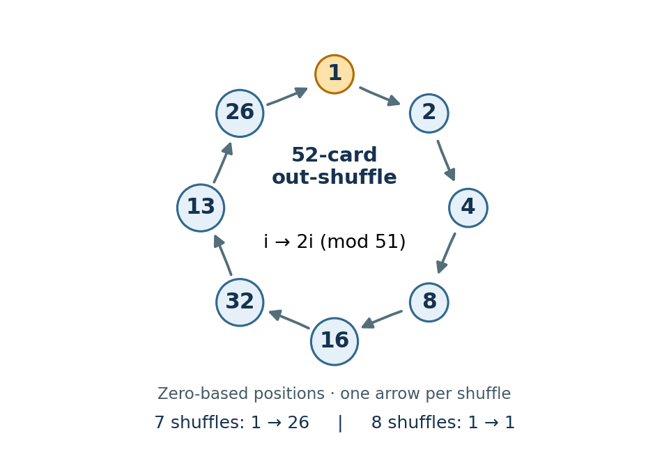
An eight-step position cycle under the 52-card perfect out-shuffle
. **Details**.

This single position already disproves a seven-step return; the modular calculation proves that the whole permutation returns after eight.

Past exam of the year 1 of the computer science course of the University of Oxford / 2022 / Functional programming, design and analysis of algorithms (resit) / 4 / c / Solution by

Codex  0 2026-10-25

Interleave equal halves, or collect the first and second components of adjacent pairs:

riffle :: [a] -> [a]
riffle = unpairs . uncurry zip . halve

unriffle :: [a] -> [a]
unriffle = unhalve . unzip . pairs

For halves as and bs of equal length, pairs (riffle xs) = zip as bs, and unzip (zip as bs) = (as,bs). Therefore unriffle (riffle xs) = xs. Conversely, starting from the adjacent pairs of any even list, separating the components, halving their concatenation and zipping them restores those same pairs. Hence riffle (unriffle xs) = xs too. Every stage takes linear time. This perfect out-shuffle leaves the first and last positions fixed.

Past exam of the year 1 of the computer science course of the University of Oxford / 2022 / Functional programming, design and analysis of algorithms (resit) / 4 / b / Solution by

Codex  0 2026-10-25

Join either two halves or successive pairs:

unhalve :: ([a],[a]) -> [a]
unhalve (xs,ys) = xs ++ ys

unpairs :: [(a,a)] -> [a]
unpairs = foldr (\(x,y) zs -> x:y:zs) []

By the defining property of splitAt, concatenating the two halves restores the original list. For unpairs, structural induction on the even input proves that its first pair restores its first two elements and the recursive result restores the rest. Thus both requested function compositions are the identity. Fully consuming either result takes at most linear time; list concatenation only copies the left half once.

Past exam of the year 1 of the computer science course of the University of Oxford / 2022 / Functional programming, design and analysis of algorithms (resit) / 4 / a / Solution by

Codex  0 2026-10-25

For finite even lists, these definitions take at most linear time:

halve :: [a] -> ([a],[a])
halve xs = splitAt (length xs `div` 2) xs

pairs :: [a] -> [(a,a)]
pairs [] = []
pairs (x:y:xs) = (x,y) : pairs xs
pairs [_] = error "pairs: odd length"

The length calculation and the prefix split each take

O (n)

time. The second operation consumes two constructors per step and emits one pair. Under the stated even-length precondition, neither definition encounters an unmatched final element.

Past exam of the year 1 of the computer science course of the University of Oxford / 2022 / Functional programming, design and analysis of algorithms (resit) / 3 / g / Solution by

Codex  0 2026-10-25

A compatible Ord instance supplies a total order, so use comparison sort to put equal values together in

O (n lo g n)

time and then group adjacent equals in linear time. To preserve the first-occurrence group ordering of part (f), first tag every element with its original index and stable sorting by value. Group the sorted records by value; stability preserves their internal input order. Each group's first record carries its smallest original index. Sort the groups by that index and finally remove the tags. The second sort has at most

n

records, so the total remains $O (n lo g n)$ time and

O (n)

storage. Merely returning the value-sorted groups could reorder the classes, so the index step matters when preserving the exact earlier convention. The stronger interface evades the equality-only lower bound by permitting order comparisons.

Past exam of the year 1 of the computer science course of the University of Oxford / 2022 / Functional programming, design and analysis of algorithms (resit) / 3 / f / Solution by

Codex  0 2026-10-25

Choose the first unclassified element as the next equivalence class representative:

equiv :: Eq a => [a] -> [[a]]
equiv [] = []
equiv (x:xs) = (x:same) : equiv rest
  where ~(same,rest) = partition (== x) xs

Assume the Eq instance is an equivalence relation. The stable list partition collects every later occurrence equivalent to x, and rest contains none of that equivalence class. Induction therefore gives exactly one group per class, preserving order within each group and ordering groups by their first occurrence. For

d

distinct classes, each input element is tested against at most

d

representatives: the cost is

O (n d)

and $Θ (n^{2})$ in the all-distinct worst case; a single class takes

Θ (n)

The equality-only grouping lower bound shows that this worst case is unavoidable in the unrestricted equality-oracle model. On an all-distinct input, an untested pair could instead be equal without changing any observed comparison. Certifying that all

n

elements belong to different classes therefore requires all

(2 n)

pairwise equality tests.

Past exam of the year 1 of the computer science course of the University of Oxford / 2022 / Functional programming, design and analysis of algorithms (resit) / 3 / e / Solution by

Codex  0 2026-10-25

Share the recursive pair and inspect the predicate once:

partition :: (a -> Bool) -> [a] -> ([a],[a])
partition _ [] = ([],[])
partition p (x:xs)
  | p x       = (x:yes,no)
  | otherwise = (yes,x:no)
  where ~(yes,no) = partition p xs

For a finite list, structural induction establishes that yes and no are the two required filtered subsequences. The guard evaluates p x once and prepends x to exactly one output, preserving input order in both. Fully consuming both results uses

n

predicate applications and

Θ (n)

additional work. Sharing the recursive result avoids making separate recursive traversals. This is a stable list partition.