
The Dijkstra algorithm solves the single-source shortest path problem in a finite graph with nonnegative edge weights, finding distances to all reachable vertices. Start with tentative distance and elsewhere. Repeatedly choose the unfinalized vertex with least tentative distance, declare that label permanent, and perform edge relaxation on its outgoing edges. For an undirected graph, inspect both directions. A finite tentative distance always records the cost of a discovered graph path, but can improve before finalization.
In our example, finalizing discovers at , at , and at . Choose next: edge relaxation through lowers to and to . Choose : edge relaxation through lowers to . Finally choose . The permanent distances are therefore , , , ; the evolving tentative distances were and .
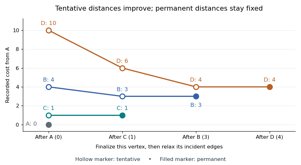
Tentative distances fall until the Dijkstra algorithm makes each label permanent
. Details. 
Store a shortest-path predecessor whenever edge relaxation improves a label. The final table contains enough information to reconstruct routes, rather than merely their costs:
| Vertex | Distance from | Shortest-path predecessor | Finalization order |
|---|---|---|---|
| None: source | |||
Following shortest-path predecessors backwards gives ; reversing the order gives . If only this destination matters, stop when is finalized. Stopping when is first discovered would incorrectly return . If the smallest remaining tentative distance is , all remaining vertices are unreachable.
Why is the permanent choice safe? Suppose the selected vertex had a cheaper graph path. Let be the first unfinalized vertex on that graph path. Its preceding vertex was finalized, so edge relaxation has already offered a label no larger than that prefix's cost. Nonnegative remaining edge weights make the whole cost at least this prefix's cost; selection gives . A cheaper graph path would contradict these comparisons. Zero weights are allowed; ties can be resolved arbitrarily. This is the reason the label-setting shortest-path algorithm works, rather than a lucky feature of the drawing.
Negative weights break that reasoning. In a directed graph with costing , costing , and costing , the Dijkstra algorithm would finalize at before discovering the cheaper cost . The Bellman-Ford algorithm handles negative edge weights when no relevant negative directed cycle exists.
With an adjacency list and an indexed binary heap implementing a priority queue, the time complexity is for , using Big O notation. Each vertex is extracted at most once, each edge is inspected once per direction, and each successful edge relaxation decreases a heap key in time. This assumes constant-cost arithmetic and comparisons; exact computation with very large weights adds their representation cost. The queue uses space beyond the graph. Simply scanning all remaining vertices gives instead.[ref]
https://algs4.cs.princeton.edu/44sp/DijkstraSP.java.html. Princeton, DijkstraSP implementation
[ref]https://algs4.cs.princeton.edu/code/javadoc/edu/princeton/cs/algs4/IndexMinPQ.html. Princeton, indexed binary heap operations
The 1959 paper presents the shortest path problem as its second problem, after the minimum spanning tree problem, and grows known shortest routes in increasing distance order.[ref]
https://www.cs.yale.edu/homes/lans/readings/routing/dijkstra-routing-1959.pdf. Dijkstra, A note on two problems in connexion with graphs, pp. 269–271
In his later recollection, Dijkstra dated the shortest-route discovery to 1956: a demonstration for the ARMAC computer used a simplified Dutch railway map and printed the route between towns. A practical request became an enduring algorithm because the same distance rule applies to any suitable graph.[ref]https://garfield.library.upenn.edu/classics1983/A1983QA19900001.pdf. Dijkstra's recollection, published in 1983
New to topics? Read the docs here!