 Fourier analysis

Fourier analysis describes a function by the oscillations that compose it. A graph records values at successive positions or times; a frequency spectrum records how much of each frequency is present, together with its wave phase. The same complicated shape can become a short list of simple components. For periodic functions, the components form a Fourier series; on the whole real line, the Fourier transform uses a continuous range of frequencies, and the Fourier inversion theorem puts them back together.

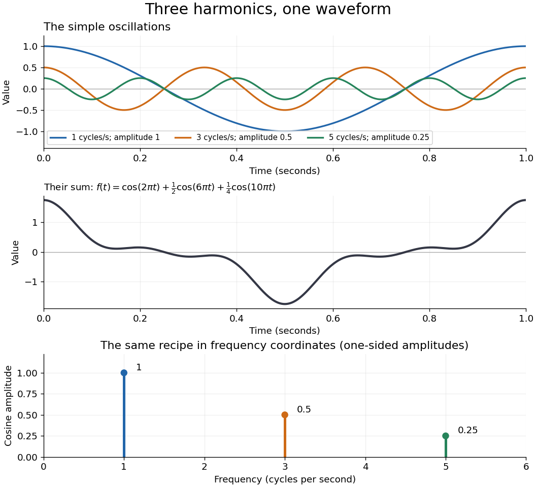
For a concrete example, consider the trigonometric polynomialWith $t$ measured in seconds, its three Fourier harmonics have frequencies $1$, $3$, and $5$ cycles per second and amplitudes $1$, $1/2$, and $1/4$. Each cosine has zero wave phase. Adding them creates the sharper peaks in the figure. The frequency spectrum makes the recipe immediately visible; changing an amplitude changes the shape without changing the component's frequency. Fourier orthogonality lets us recover each Fourier coefficient by averaging against the corresponding sine or cosine, because the other Fourier harmonics cancel over a full period of a function.

The deeper reason these components are so useful is that they simplify operations. By Euler's formula, the exponential function $e^{i\omega x}$ packages a cosine and a sine into one Fourier mode. A translation or a derivative changes only its multiplier:Thus Fourier modes are simultaneous eigenfunctions of these operations. In Fourier series, this gives a literal diagonalization in the Fourier basis; on the real line, the Fourier transform gives the continuous counterpart, with each frequency handled separately. The Translation property of the Fourier transform and the Fourier transform of a derivative turn shifting and differentiating a whole function into multiplication of its Fourier transform. A convolution likewise becomes multiplication by the convolution theorem. This is beautiful because one description simplifies several apparently different operations at once.

For example, the heat equation $u_t=\kappa u_{xx}$, with thermal diffusivity $\kappa >0$, evolves a spatial Fourier mode asFine ripples have larger angular frequencies and decay faster: the formula explains why heating smooths a jagged temperature profile. For a general initial profile with sufficient regularity, the Fourier transform gives $\hat{u}(\omega ,t)=e^{-\kappa {\omega }^{2}t}\hat{u}(\omega ,0)$, and Fourier inversion recovers the temperature. Similarly, multiplying selected parts of a frequency spectrum suppresses unwanted components. Claude E. Shannon's Communication in the Presence of Noise (1949), Section III, describes ideal filtering as a projection that retains some frequency coordinates and removes others.^[ref]

The physical motivation is already visible in Joseph Fourier's Théorie analytique de la chaleur (1822). Chapter III constructs heat profiles using sums of sines and cosines; Chapter IX, articles 355–359, passes from Fourier series to integrals as the spatial interval becomes unbounded. These heat problems explain the motivation for the discrete and continuous descriptions. Their modern formulations specify which functions admit reconstruction and in what sense the expansions converge.^[ref][ref]

Fourier analysis is a mathematical technique used to analyze functions or signals by decomposing them into their constituent frequencies. Named after the French mathematician Jean-Baptiste Joseph Fourier, this method is based on the principle that any periodic function can be expressed as a sum of sine and cosine functions (Fourier series) or, more generally, as an integral of sine and cosine functions (Fourier transform) for non-periodic functions.