Homogeneous linear differential equation
ID: homogeneous-linear-differential-equation

A homogeneous linear differential equation is a linear differential equation with identically zero forcing term, . On a common interval, its solutions of a differential equation form the vector space , the kernel of a linear map. They include the zero function and are closed under addition and scalar multiplication. For any two solutions of a differential equation and constant scalars , linearity gives : this is the superposition principle. The scalars must be constant; variable multipliers introduce extra derivatives.
For example, has general solution , where is any constant real number. A short verification uses the product rule: , so is constant. For and , the sum is and also solves the same homogeneous linear differential equation. At , their values are approximately , and . Every curve is a multiple of one exponential function; the solution space of a homogeneous linear differential equation has dimension one. Both and in this example and the following diagram are dimensionless mathematical variables.
Now keep the same differential operator but prescribe the forcing term . The inhomogeneous linear differential equation has particular solution and general solution . The initial conditions select, respectively,At , their values are approximately , and . The midpoint solves the same inhomogeneous linear differential equation, because . The sum instead satisfies , so it fails the equation with forcing term . More generally, a linear combination of solutions of a differential equation for the same fixed nonzero forcing term retains that forcing term precisely when its scalar weights add to one. This is the affine space structure, rather than unrestricted superposition within that fixed family.
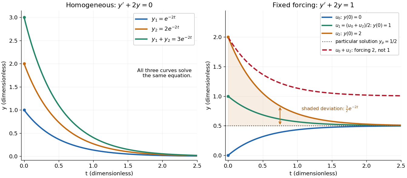
Homogeneous solutions obey superposition, while a fixed forcing term gives a particular solution plus homogeneous solutions
. Details. 
On the left, all three curves solve the same homogeneous linear differential equation. On the right, share the particular solution , and the shaded difference is the homogeneous solution . The dashed sum has twice the forcing term, even though its starting value coincides with that of . Adding the two initial conditions also adds their inputs; taking their midpoint averages both. This distinction makes the superposition principle useful for assembling responses to different inputs without mistaking that assembly for a solution of a differential equation with the original input. See MIT's superposition notes, including the particular solution one half.
New to topics? Read the docs here!