A vector space over a field is a set equipped with vector addition and scalar multiplication satisfying the vector space axioms. Its vectors can represent directed displacements, lists of measurements, polynomials, or entire functions. The common structure is that adding two elements and multiplying an element by a scalar remain meaningful operations inside the same space.
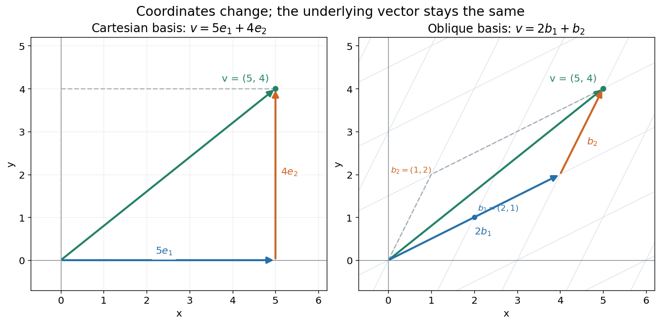
For example, uses coordinatewise addition and scaling. Withwe have . Moving twice along and once along reaches the same vector as five horizontal and four vertical steps. The two descriptions refer to different bases of the same space. A basis makes such descriptions unique; a spanning set makes them possible.
The space of real polynomials of degree at most two has basis : the polynomial is the linear combination with coordinates . The zero vector here is the zero polynomial, and addition combines coefficients. A derivative is a linear map on this space; its matrix records how it acts on the three basis vectors. The same coordinate machinery therefore handles both geometric motion and operations on functions.
The choice of field matters. The complex numbers form a one-dimensional vector space over with basis , but a two-dimensional vector space over with basis . The question "how many independent directions?" has an answer only after the allowed scalars are specified. Likewise, polynomials of degree exactly two do not form a vector space: subtraction can remove the leading term, and the zero polynomial is absent.
The usefulness of the abstraction is that a linear map is determined by its values on a basis. Once those images are known, linear combinations give its action on every vector. The rank-nullity theorem relates the number of attainable outputs to the number of invisible input directions, while change of basis lets us choose coordinates suited to the problem. Eigenvectors, for example, choose directions on which repeated application of a linear operator becomes scalar multiplication.
A historical source is Hermann Grassmann's Die lineale Ausdehnungslehre (1844). Its full title advertises applications to other branches of mathematics, statics, mechanics, magnetism and crystallography; the original edition is digitized by ETH-Bibliothek. This gives an early setting for treating geometric quantities algebraically across different applications, rather than attributing the modern axiom list to that title alone.[ref]
https://www.e-rara.ch/zut/content/titleinfo/1169335. Grassmann, Die lineale Ausdehnungslehre, Leipzig, 1844; ETH-Bibliothek Rar 5128
Addition makes an Abelian group: for all , and , there is a zero vector , and every has an additive inverse . Scalar multiplication satisfies, for ,Both operations take values in . These requirements make manipulating linear combinations independent of how sums are grouped or expanded.
A sequence space is a vector space of scalar sequences, closed under coordinatewise addition and scalar multiplication. Examples include the l-p sequence space, the l-infinity sequence space and spaces of convergent sequences.
The zero vector of a vector space is its additive identity: for every vector . It is unique, because if is another such identity then . Distributivity gives , so after cancellation. In a coordinate vector space it has every coordinate zero.
A vector space with scalar field is equivalently a torsion-free divisible Abelian group. An embedding of such groups automatically respects rational scalar multiplication because solutions to are unique.
For complex vector spaces, an antilinear map satisfies . It is linear over the real numbers and conjugates complex scalar multiplication. This differs from two conjugate linear operators, which are related by similarity rather than conjugate-linearity.
An antilinear endomorphism with square equips a complex vector space with a quaternionic structure: complex multiplication supplies the quaternionic generator and supplies , satisfying . Such a space has even complex dimension. There is no invariant complex line, because would imply . In dimension four the invariant complex two-planes are quaternionic lines, forming . This is the Euclidean reality structure on twistor space used in twistor theory.
An antiunitary operator between complex Hilbert spaces is a surjective antilinear map satisfying the displayed inner product identity. It preserves norms but conjugates scalars. In a chosen orthonormal basis it is , with a unitary operator and coefficientwise complex conjugation. Conversely any such is antiunitary. Antilinearity by itself does not preserve norms.
A vector space over the field of complex numbers. A complex-linear map preserves addition and multiplication by complex scalars.
For real vectors of equal length and equal sum, write when for every proper initial segment; the downward arrow means decreasing rearrangement. Majorization compares how unevenly a fixed total is distributed. The uniform probability vector is majorized by every probability vector, while majorizes every probability vector. The order controls exact pure-state entanglement conversion in Nielsen's pure-state conversion theorem.
For decreasing positive sequences in , write if every initial partial sum of is at most the corresponding partial sum of and the finite total sums agree. The finiteness requirement matters: equality of two divergent totals interpreted as infinity is too weak to guarantee a doubly stochastic realization of summable-sequence majorization.
Decreasing strictly positive summable sequences with equal totals and admit an infinite doubly stochastic matrix realizing the displayed relation. Choose with and average the pair to obtain and . The remaining decreasing sequence majorizes the remaining target sequence: short initial sums contain values at least , and longer sums are the old sums minus . Repeat on the tail, freezing one normalized finite-support row at each stage. Limit column sums are at most one; Tonelli's theorem, equal finite totals and strict positivity of every force every column sum to equal one.
If is a finite field, a vector space of finite dimension over has elements. Every infinite-dimensional vector space over is an infinite elementary abelian -group under addition.
A subset of is a finite-field Kakeya set when it contains an affine line in a vector space in every one-dimensional direction. The line position may depend on the direction. The polynomial method in combinatorics yields the finite-field Kakeya polynomial bound on its cardinality.
For odd characteristic, the union of the lines contains a line of every finite slope. For fixed , completing the square shows that it comprises the values of for which is a square, including zero. Adding the vertical line completes the directions and gives cardinality . This is a finite-field Kakeya set whose density tends to one half.
For a finite-field Kakeya set , a smaller cardinality would give a nonzero polynomial of total degree of a polynomial at most vanishing on , by the dimension of a bounded-total-degree polynomial space. Its restriction to each complete affine line in a vector space has roots of a polynomial and degree less than , hence vanishes identically. The top homogeneous polynomial part then vanishes in every direction. A polynomial of degree less than in each variable cannot vanish everywhere on unless it is zero, giving a contradiction. For the prime field, this is the polynomial nonvanishing below the field size.
The linear span of a subset of a vector space is the set of all finite linear combinations of elements of . It is the smallest vector subspace containing : every vector subspace containing the original vectors must contain their sums and scalar multiples.
In , the linear span of is a line, the linear span of is the plane , and adding gives all of . Adding to the first set changes none of its attainable vectors, because it is already a scalar multiple of . Thus a spanning set can contain redundant generators; linear independence identifies when this redundancy is absent. In an infinite-dimensional space, an algebraic linear span still uses finite sums; a closed linear span can also include limits in a specified norm.
In a normed vector space, the closed linear span of is the closure of its linear span in the norm topology. It includes limits of finite linear combinations. In a Hilbert space, an infinite orthonormal basis spans in this closed sense, allowing norm-convergent series in addition to finite sums.
For a vector subspace , the quotient vector space consists of cosets , with vector operations induced from .
For fixed , the parallel affine lines are precisely the cosets of the indicated quotient vector space. Changing representatives adds a multiple of , so and are well-defined. The zero is the whole line , not a single point. If is a basis, the two line classes form a basis of the quotient by spanning and independence modulo .
A vector subspace is a nonempty subset of a vector space closed under vector addition and scalar multiplication, and is therefore itself a vector space. Equivalently, whenever belong to the subset, so does for all allowed scalars . In particular it contains the zero vector.
For example, the plane is a vector subspace, with basis . Indeed every element is . The parallel plane misses the zero vector and is an affine subspace instead. Homogeneous constraints produce vector subspaces: is the kernel of the linear map . This lets us describe all solutions of a homogeneous linear equation through a basis of its kernel.
A proper vector subspace of a vector space is one strictly smaller than the ambient space. In a finite-dimensional vector space, this is equivalent to having smaller dimension: a basis of the subspace can be extended to a basis of the ambient space, and strict inclusion requires at least one additional vector.
A flag is a strictly nested chain of vector subspaces of a fixed vector space. A complete flag contains a subspace of every possible dimension. For an action by linear maps, an invariant flag means that each of its vector subspaces is an invariant subspace. A basis adapted to an invariant complete flag makes all these maps upper triangular, connecting complete flags to simultaneous triangularization of a Lie algebra representation.
A complete flag in an -dimensional vector space is a nested sequence of vector subspaces with . An action preserves such a flag exactly when its matrices are upper triangular in a basis adapted to the flag. The Lie theorem supplies an invariant complete flag for every complex finite-dimensional Lie algebra representation of a solvable Lie algebra.
The fixed coordinate subspace of dimension in consists of vectors whose coordinates after the first vanish. Restricting a quadratic form to it uses only the leading by matrix block. It specifies one fixed support; allowing every support of size would introduce another combinatorial counting step.
The intersection of any family of vector subspaces of a common vector space is the set of vectors belonging to every member of the family. It is again a vector subspace.
A hyperplane is a vector subspace of codimension one. A projective hyperplane in is the zero set of one nonzero homogeneous linear form.
A closed vector subspace of a topological vector space is both a vector subspace and a closed set. The kernel of a continuous linear map is a closed vector subspace.
If is a nonzero closed linear subspace of a normed ambient space and is finite-dimensional with , the unit sphere of has positive distance from . Otherwise a sequence of nearly coincident points yields a bounded sequence in , hence a convergent subsequence; closedness of puts its norm-one limit in both vector subspaces. In applications to a bidual space, completeness of the Banach space makes its canonical image closed.
An affine subspace of a vector space is a translate of a vector subspace . Its dimension is the dimension of .
The smallest affine subspace containing a nonempty set . For any chosen , the displayed formula proves existence and minimality: every containing affine subspace must contain all the indicated differences in its direction space. Equivalently it consists of finite affine combinations with . Its dimension can be smaller than the dimension of an affine hyperplane in which the set has been embedded.
In a finite-dimensional real vector space, a level set of a nonzero linear functional is an affine hyperplane. Choosing in that level set gives , so its dimension is one less than that of the ambient space. With a Euclidean inner product, translation followed by an orthonormal basis of identifies it isometrically with the lower-dimensional Euclidean space. The coordinate-sum constraint on balanced cut vectors is an example.
In a vector space over a field , an affine line is a translate of a one-dimensional vector subspace. Its direction is that vector subspace, so multiplying by a nonzero scalar preserves the direction. Over a finite field of size it contains exactly distinct points. This usage concerns affine subsets of vector spaces, rather than the affine line as an affine scheme.
Let be a vector space over a specified field , and let . A linear combination is a finite sumThe coefficients are scalars from that same field; each term uses scalar multiplication, and the terms are joined by vector addition. For coefficients in the real numbers, negative values reverse arrows and fractional values scale them by fractional amounts. The collection of attainable vectors is the linear span. The column picture in Strang's MIT notes interprets solving a linear system as choosing coefficients to reach a target vector.[ref]
https://ocw.mit.edu/courses/18-06sc-linear-algebra-fall-2011/6913aa2f37dada8fdda334168b30339b_MIT18_06SCF11_Ses1.1sum.pdf. MIT 18.06SC, Strang lecture summary 1, pp. 2–3: the column picture
For a concrete calculation over the real numbers, takeThen . More generally, solving and givesEvery vector in the Euclidean plane is therefore a linear combination of , so their linear span is all of . The target has coefficients ; the target has coefficients , since . The displayed formula also makes the coefficients unique. Consequently is an ordered basis, with coordinate vector .
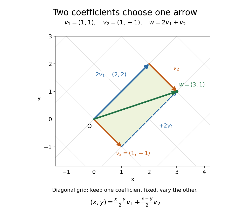
The payoff is a reusable language for synthesis: linear combinations build vectors from chosen ingredients, linear span decides which targets are reachable, and linear independence decides whether the coefficients are unique. The ingredients can also be polynomials or functions, as long as they belong to a vector space over the specified field.
An integer linear combination is a linear combination whose coefficients are integers. The lattice basis definition uses unique integer linear combinations, rather than arbitrary real coefficients. For example, is a real linear combination of but is not an integer linear combination of that single vector.
A scalar multiplying a specified term in a linear combination, polynomial or power series. When the term family has linear independence, the coefficients are unique; uniqueness of finite Laurent polynomial coefficients follows after multiplying by a sufficiently large power to obtain an ordinary polynomial.
Vector addition is the vector space operation combining two vectors into their sum. It is commutative and associative, has the zero vector as identity, and distributes with scalar multiplication as specified by the vector space axioms. Coordinatewise addition describes it after choosing a basis.
The dimension of a vector space is the cardinality of any of its bases. In finite dimension this counts the scalars needed to specify an arbitrary vector once an ordered basis is chosen. The exchange argument behind the basis extension theorem shows that any two finite bases have the same size: an independent family cannot be larger than a spanning family.
Thus has dimension two even with an oblique basis, has dimension three, and the homogeneous plane in vector subspace has dimension two. This count concerns independent freedom, so an embedded plane remains two-dimensional while sitting in a three-dimensional ambient vector space. Dimension also depends on the field, as the two interpretations of in vector space illustrate.
The direct sum of two vector spaces consists of pairs with componentwise operations. A vector space is an internal direct sum of subspaces and exactly when every vector has a unique expression with and .
If with nonzero subspaces, choose and write using the first direct sum of vector spaces. Both components are nonzero. The plane spanned by them meets and in their component lines and meets in the line through . Its intersection with cannot be the whole plane, since .
An orthogonal direct sum is a direct sum whose distinct summands are mutually orthogonal. For and , the Pythagorean identity gives . In a Hilbert space, a closed subspace of a Hilbert space and its orthogonal complement give an orthogonal direct sum of the entire space. The component maps are orthogonal projections and have operator norm one when their ranges are nonzero.
A submodule of a module is a direct summand if some submodule gives . Equivalently, the inclusion has a left inverse R-module homomorphism, or is the image of an idempotent endomorphism of .
Integer row vectors forming a square unimodular matrix are a basis of the corresponding free abelian group: the adjugate formula makes the inverse integral. The subgroup spanned by any subset of that basis is therefore a direct summand, complemented by the remaining basis vectors. In contrast, a proper finite-index subgroup of a free abelian group cannot be a direct summand: its nonzero finite quotient would have to embed as a subgroup of a torsion-free group.
For every subspace of a finite-dimensional vector space , extending a basis of to a basis of produces a subspace such that .
In a vector space over a specified field , a finite family of vectors is linearly independent when, for coefficients ,Here the left-hand zero is the zero vector, while the right-hand zeros belong to the field . Thus linear independence excludes every nontrivial linear relation. For an infinite family, require this condition for every finite subfamily.[ref]
https://ocw.mit.edu/courses/18-06sc-linear-algebra-fall-2011/0bbc30e3f1d7933ea07a2d2e9ab050d9_MIT18_06SCF11_Ses1.9sum.pdf. MIT 18.06SC, Strang lecture summary 9, p. 1: linear independence
For and over the real numbers, the linear relation gives and . Adding and subtracting yields , hence . This verifies linear independence directly and explains why the linear combination giving has exactly the coefficients .
A linearly independent family cannot contain the zero vector: a coefficient of on that entry and on every other entry would be a nontrivial linear relation. The empty family is linearly independent, because its empty sum is the zero vector and there are no coefficients that could be nonzero. Linear independence identifies a collection without redundant vectors; combined with a spanning set, it gives a basis. The uniqueness of linear combination coefficients makes its representations unambiguous.
A family is linearly independent if and only if every vector in its linear span has unique coefficients as a linear combination of that family. For a short proof, subtract two representations to get ; linear independence forces each difference to vanish. Conversely, uniqueness applied to the zero vector forces every linear relation to use only zero coefficients. This explains the practical role of linear independence: a coordinate vector relative to an ordered basis is unambiguous.
A finite vector family is minimally dependent if it is linearly dependent and every proper subfamily is linearly independent. For , the family in is an example. The sum supplies a nonzero dependence. If the sum vector is omitted, the remaining vectors are a coordinate basis; if is omitted, its coordinate in any proposed relation forces the coefficient of the sum vector to vanish, then all other coefficients vanish. Every smaller proper subfamily lies in one of these independent -element subfamilies.
Let the first columns of a matrix be the first dependent prefix, with no zero column. Their relation space has dimension one, and every nonzero relation has at least two nonzero coordinates. If both and , one-dimensionality gives for all . Two nonzero coordinates would force two of the distinct weights to agree, a contradiction.
A finite family of vectors in a vector space over a specified field is linearly dependent if it has a nontrivial linear relation: with and at least one coefficient nonzero. One can then solve for a vector whose coefficient is nonzero as a linear combination of the others; removing that entry preserves the linear span. Repeated vectors in a list give linear dependence: for example has the linear relation . A list keeps both entries even though the set has only one element. Strang's notes illustrate redundant columns by expressing one as the sum of two others.[ref]
https://ocw.mit.edu/courses/18-06sc-linear-algebra-fall-2011/0bbc30e3f1d7933ea07a2d2e9ab050d9_MIT18_06SCF11_Ses1.9sum.pdf. MIT 18.06SC, Strang lecture summary 9, pp. 2–3: dependent columns
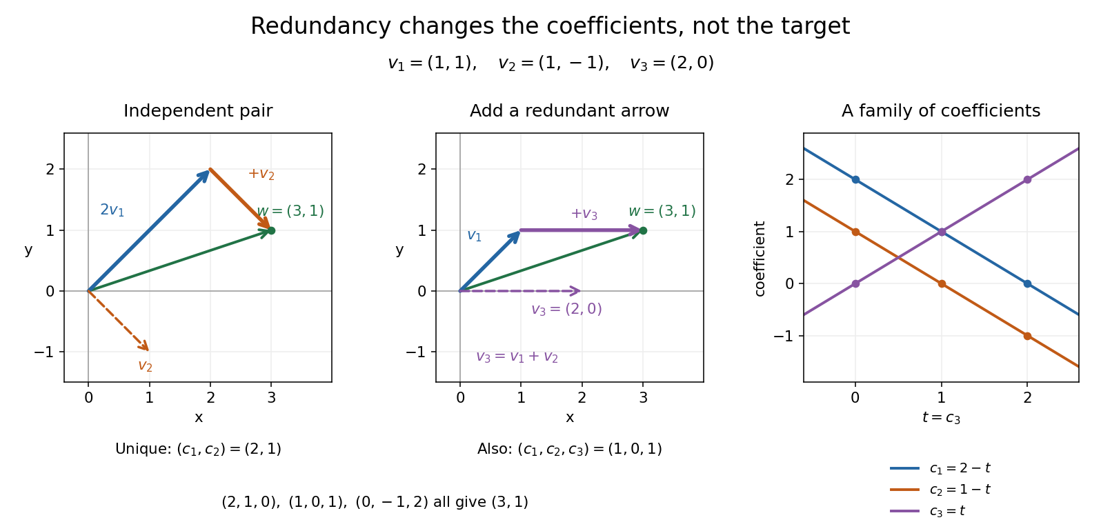
Keep and , and add . The three vectors still have linear span , but nowThe two coefficient triples and differ by the nontrivial linear relation . In fact all linear combination representations of this target areTo check both completeness and correctness, use . Linear independence of forces and , giving exactly the displayed family. Redundancy therefore preserves attainable targets while allowing their coefficients to move. For solving a linear system, these alternatives matter; for assigning unique coordinate vectors, one instead chooses a basis.
The following example shows why linear independence depends on the scalar field.
Consider the vectors in the complex numbers, where is the imaginary unit. With scalar field , a linear relation has . Taking its real part and imaginary part gives , so the pair is linearly independent. Every complex number also has coefficients in the real numbers, so form a basis and the dimension of a vector space is two.
With scalar field , the same pair is linearly dependent, sinceuses the nonzero coefficients from the complex numbers. The single vector is now a basis, because for every complex number , giving dimension of a vector space one. For example : the second representation uses a coefficient unavailable over the real numbers. Specifying the field is part of the definition of linear independence.
A linear relation among vectors is a coefficient tuple satisfying . It is nontrivial if at least one coefficient is nonzero. For the matrix with these vectors as columns, the space of relations is its kernel. The vectors are linearly independent exactly when this kernel is zero. An invertible change of coordinates preserves every relation, since if and only if .
A basis is a linearly independent spanning set of vectors in a vector space. Every vector is a unique finite linear combination of basis vectors. Independence supplies uniqueness, and spanning supplies existence. An ordered basis turns the coefficients into a coordinate vector.
For , the matrix with these vectors as columns isHence the coordinate vector of is , and recovers the usual coordinates. The determinant is nonzero, so this recovery works for every vector in . A basis need not have perpendicular or unit-length vectors; an orthonormal basis adds those geometric conveniences when an inner product is available.
The point of changing basis is to simplify the operation being studied. Diagonalization uses an eigenbasis to turn a coupled linear map into independent scalings. In a space of polynomials, the basis makes differentiation easy to encode, while orthogonal polynomials can make approximation errors easier to measure. Gilbert Strang's MIT lecture on independence, basis and dimension develops this connection between attainable columns, redundant columns and coordinates.[ref]
https://ocw.mit.edu/courses/18-06sc-linear-algebra-fall-2011/. Strang, MIT 18.06SC, Independence, Basis and Dimension
An ordered basis is a basis equipped with an ordering of its basis vectors. The order fixes which position of a coordinate vector corresponds to each basis vector.
For an ordered basis , the coordinate vector records the unique coefficients satisfying . Change of basis changes this representation while preserving the underlying vector.
For , , the vector has coordinate vector , since . These are the same coefficients extracted by the dual basis in its worked example. The vector is independent of the chosen basis; its list of coordinates is not. In an orthonormal eigenbasis, the coordinates additionally separate the action of a self-adjoint operator into independent scalar multiplications.
A coordinate of a vector in a chosen basis is one entry of its coordinate vector. The corresponding coordinate functional in the dual basis extracts it. For an orthonormal basis, it can instead be read as an inner product with the basis vector, as in orthonormal eigenbasis. For a nonorthogonal basis, ordinary dot products need not give the coordinates.
A basis vector is one of the vectors in a specified basis of a vector space. Its coordinate column in that basis has one entry equal to one and all other entries zero. Columns of a matrix of a linear map are the images of domain basis vectors, expressed in the chosen codomain basis.
For a basis with cyclic indexing, the vectors have coefficient matrix , where cyclically shifts coordinates. Its determinant is . They therefore form a basis exactly when is odd over a field of characteristic different from two. For even , alternating coefficients produce a nontrivial linear dependence.
Every linearly independent subset of a finite-dimensional vector space extends to a basis. Starting with its vectors, add a vector outside their current span until the span is the whole space. Each addition preserves linear independence, and the process stops because the dimension is finite. This also lets a linear functional on a vector subspace extend to the ambient space by assigning arbitrary values on the additional basis vectors.
The standard basis of the vector space consists of the vectors whose th coordinate is one and whose other coordinates are zero. Every vector has the unique expression in this basis.
If a vector space is spanned by vectors, every linearly independent family in it has at most members. Consequently, any two finite bases have the same number of vectors.
For polynomials in fixed variables and of a fixed degree, the monomials of that degree form a basis of the corresponding homogeneous component.
A vector is an element of a vector space. Its defining operations are vector addition and scalar multiplication. An arrow in a Euclidean space is one example; a polynomial or a function can also be a vector when the chosen vector space uses the corresponding addition and scalar multiplication.
For instance, the polynomials and belong to the real vector space of polynomials of degree at most two. Their vector addition gives , and scalar multiplication gives . In the monomial basis these are the coordinate vectors , , and respectively. The vectors are the polynomials; these tuples are their representations in a chosen basis.
A general vector space does not itself prescribe lengths or angles. A norm supplies a size, while an inner product also supplies angle information and orthogonality. The familiar arrow geometry below belongs to Euclidean vectors, where this extra structure is available.
An axial vector transforms as under an orthogonal matrix . It agrees with a polar vector under a proper rotation matrix and has the additional determinant sign under an orientation-reversing transformation. Angular momentum and angular velocity are axial vectors.
A polar vector transforms as under an orthogonal matrix , including an orientation-reversing transformation. Displacement, velocity and force are polar vectors. An axial vector instead transforms as .
A Euclidean vector is a vector in a finite-dimensional real inner product space. Choosing an orthonormal basis identifies it with its real vector components in . A geometric arrow represents a Euclidean vector by a length and a direction; translating the arrow without changing either represents the same Euclidean vector. The zero vector has length zero and no distinguished direction.[ref]
2.1 Scalars and Vectors. University Physics Volume 1 by William Moebs and others; §2.1, Figures 2.2–2.5: vector arrows, equal vectors and displacement
For points and in a Cartesian coordinate system, the displacement is . The arrow from to represents the same Euclidean vector, even though its endpoints differ. An endpoint is a position; their difference is a vector. In an orthonormal basis ,The Euclidean norm comes from the inner product: . The sum of squared vector components is valid in an orthonormal basis; an arbitrary basis requires the appropriate Gram matrix. This distinction lets the geometric vector stay the same while its coordinate vector changes.[ref]
2.2 Coordinate Systems and Components of a Vector. University Physics Volume 1 by William Moebs and others; §2.2, Cartesian coordinates: equations (2.10)–(2.13) and Figure 2.16, unit basis vectors and scalar components
Vector addition is componentwise. With and ,Geometrically, translate the second arrow so its tail starts at the first arrow's head. The vector sum joins the starting point to the final endpoint. Reversing the order gives the other route around the same parallelogram, so vector addition is commutative. This is the useful bookkeeping behind adding successive displacements, velocities, or forces: direction information survives the calculation. For a force, the Euclidean vector alone does not specify its point of application, which also affects the torque.[ref]
2.1 Scalars and Vectors. University Physics Volume 1 by William Moebs and others; §2.1, Algebra of Vectors in Two Dimensions: Figure 2.12 and the head-to-tail construction
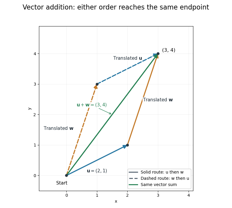
Two orders of vector addition reach the same endpoint
. The original Euclidean vectors and form a parallelogram. Either head-to-tail route gives their vector sum ; dashed copies are translated arrows, not additional terms. Details.The magnitude of a vector sum is generally different from the sum of the magnitudes. Here , whereas . The triangle inequality explains why the direct displacement cannot exceed the length of this two-segment route. A return displacement makes the net vector sum zero, although the lengths of the three travelled segments sum to a positive number.
The dot product exposes direction quantitatively: for nonzero Euclidean vectors, . For the displayed pair, the dot product is , so and the angle is . For orthogonal vectors, that dot product is zero. Dividing by magnitudes separates direction from size, which is the purpose of vector normalization.
A unit vector is a vector of norm one in a normed vector space. For a nonzero vector , vector normalization produces one by dividing by . In a real Euclidean space, this keeps the direction and removes the magnitude. The zero vector cannot be normalized because its norm is zero.
For with Euclidean norm , the corresponding unit vector isThe Euclidean vector can therefore be reconstructed as : size and direction are distinct pieces of information. The standard basis vectors are familiar unit vectors, but a unit vector need not point along a coordinate axis.
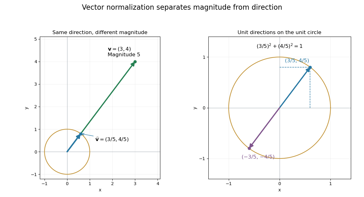
Normalization keeps direction and places the endpoint on the unit circle
. The original Euclidean vector has magnitude . Its vector normalization lies on the unit circle. The enlarged right panel also shows its negative, which has the same Euclidean norm and the opposite direction. Details.Vector normalization converts a nonzero vector in a normed vector space into a unit vector. Absolute homogeneity of a norm givesThe direction is unchanged by multiplying by a positive real scalar. For , and ; for a negative real scalar, . Thus and normalize to the same unit vector, while normalizes to its negative. This decomposition is useful for specifying a direction independently of a force, velocity or displacement magnitude.
In a complex normed vector space, a nonzero complex scalar instead gives . The remaining complex argument is not removed by normalization. For a pure quantum state, vectors differing only by this overall global phase represent the same physical state; vector normalization alone does not identify them.
Vector normalization is not a linear map. With and ,Consequently, adding individually normalized directions does not generally give the direction of the original vector sum. Compute the intended vector sum first, then normalize it if it is nonzero. Cancellation is a further boundary case: has no normalized direction even though both nonzero summands do. A numerical algorithm must check that case before dividing by the norm.
The cross product of two three-dimensional vectors is perpendicular to both, has magnitude , and is oriented by the right-hand rule.
For , maps in factor uniquely through ; maps in have image in . Thus these vector subspaces are naturally and , of dimensions and . Passing to a dual map reverses composition and interchanges these two spaces. This gives a basis-free route to equality of the ranks of a map and its dual.
For endomorphisms of the same finite-dimensional vector space, makes surjective and injective. The rank-nullity theorem makes both invertible, hence . The finite-dimensional and equal-domain assumptions matter; unilateral shift operators on an infinite-dimensional sequence space give one-sided inverses that are not two-sided.
The rank of a linear map is the dimension of its image of a linear map. In finite-dimensional spaces it equals the rank of a matrix representing the map in any bases.
The image of lies in . The dimension formula for a sum of subspaces gives the upper bound. Applying it to and then interchanging gives the lower bound. Both extremes are sharp: cancelling diagonal blocks gives the difference of ranks; diagonal maps with supports covering the whole space and positive coefficients give full rank when the sum of prescribed ranks is at least the dimension.
For a nonzero vector and nonzero linear functional vanishing on , this invertible map fixes the hyperplane pointwise and has determinant one. Its inverse is , since . A symplectic transvection is obtained by taking for a nondegenerate alternating bilinear form.
Every nonidentity transvection has an adapted basis in which it is . Thus all such maps are conjugate in the general linear group. In dimension at least three, a scaling of a third basis vector centralizes this matrix and has arbitrary nonzero determinant; adjusting a conjugator by this scaling proves conjugacy in the special linear group as well.
// Target: algebra.bigb
This matrix adds times coordinate to coordinate . Left multiplication performs the corresponding row addition. Such matrices generate the special linear group over a finite field: row elimination also realizes signed interchanges and compensating diagonal scalings using products of these matrices.
Row additions reduce an invertible matrix to diagonal form without changing determinant. A determinant-one diagonal matrix is a product of diagonal two-coordinate blocks , each expressible as a product of six elementary transvection matrices. Therefore these matrices generate the special linear group over a field.
// Target: algebra.bigb
A horizontal shear fixes the horizontal axis pointwise and sends to . Its determinant is one and both eigenvalues are one. A nonzero shear preserves area but generally changes lengths and angles. Composing a shear with a planar rotation can produce a symmetric stretch; having determinant one alone does not make a linear map a shear.
A uniform dilation about the origin multiplies every vector by one positive real scale . The linear map multiplies lengths by and -dimensional volumes by . This differs from stretching different axes by different factors. The case is the identity map.
A real-linear map between complex vector spaces that commutes with multiplication by . On , its real matrix is , representing multiplication by . On , such a map with real determinant one is a rotation. In higher complex dimension, determinant one does not force the map to be a unitary operator.
If a linear functional vanishes on the image of a linear map but , the equation has no solution. In Euclidean coordinates, a vector with provides such an obstruction whenever . In finite dimensions these annihilating functionals exactly characterize membership in the image: precisely when it is orthogonal to every vector in .
A linear map is surjective when its image is all of . For finite-dimensional spaces this is equivalent to .
This is a scalar-valued linear functional, so it vanishes at the origin; an affine function with a nonzero constant term is a different notion.
An affine function on a real or complex vector space has the form , where is a linear map and is constant. Its derivative is the constant map . It is linear exactly when .
Linearity is the property .
Articles were limited to the first 100 out of 209 total.
Articles by others on the same topic

This is a section about Vector space!
For example, this sentence. And then another one.

This is a section about Vector space!
For example, this sentence. And then another one.

A vector space (or linear space) is a fundamental concept in mathematics, particularly in linear algebra. It consists of a collection of objects called vectors, which can be added together and multiplied by scalars (numbers). These operations must satisfy certain properties.



