Known-variance Gaussian mixture EM example
ID: known-variance-gaussian-mixture-em-example

Choose six illustrative values , fixed mixture weights , known standard deviation , and initial means . These are constructed data for a Gaussian mixture distribution, not measurements. With the standard normal distribution probability density function, the fitted log-likelihood isAt the initial means, the component density ratio is . The first E-step therefore gives
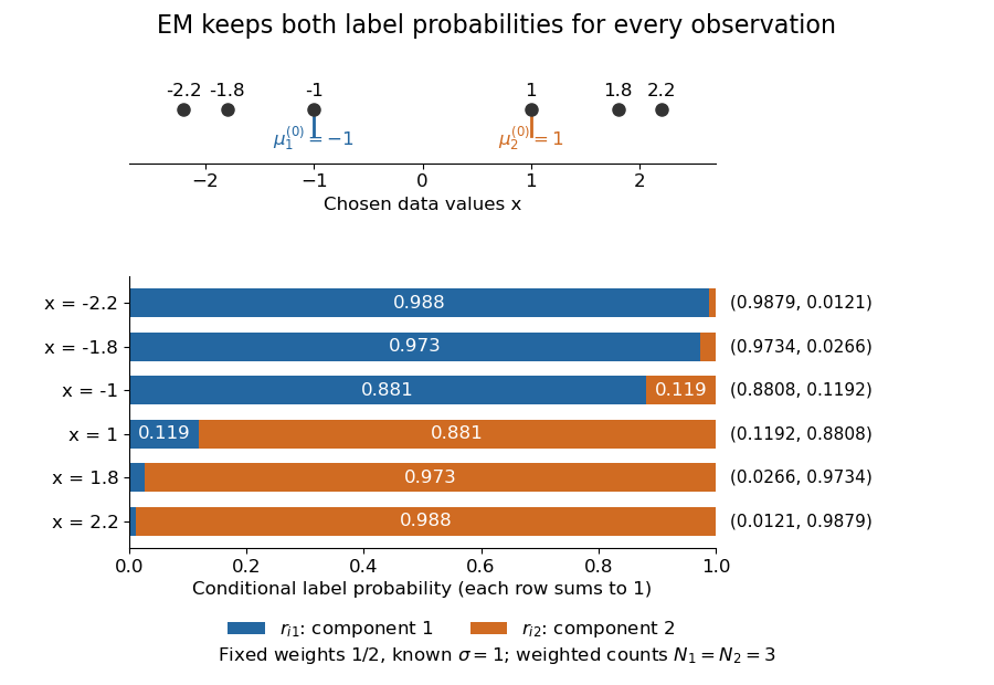

The paired values and have complementary mixture responsibilities, so exactly. The first M-step givesThe hyperbolic tangent expression follows by pairing the contributions at and . Assigning every negative value wholly to the first mixture component and every positive value wholly to the second would instead give means . Those hard assignments discard the overlap: the expectation-maximization algorithm is not the same update as K-means clustering.
The observed-data log-likelihood rises from initially to after one update and after two. Further updates approach means , with log-likelihood approximately . These values describe this initialization; EM likelihood monotonicity supplies no certificate of a global maximum.
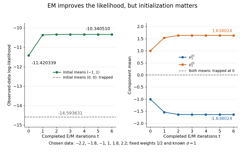
Likelihood ascent and mean updates for the chosen data, compared with an identical-means initialization
. Iteration zero is the initial fit; each subsequent point follows one E-step and one M-step. Starting at minus one and one increases the likelihood. Starting both means at zero leaves them at zero with a lower constant likelihood. All runs keep variance one and weights one half. Details.
For stable numerical evaluation, put and . The log-sum-exp function givesSubtracting keeps at least one exponential equal to one, avoiding the all-zero sum that direct evaluation of tiny component densities can produce.
New to topics? Read the docs here!