Choose six illustrative values , fixed mixture weights , known standard deviation , and initial means . These are constructed data for a Gaussian mixture distribution, not measurements. With the standard normal distribution probability density function, the fitted log-likelihood isAt the initial means, the component density ratio is . The first E-step therefore gives
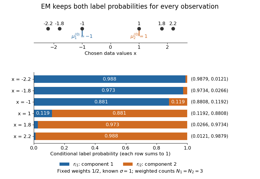

The paired values and have complementary mixture responsibilities, so exactly. The first M-step givesThe hyperbolic tangent expression follows by pairing the contributions at and . Assigning every negative value wholly to the first mixture component and every positive value wholly to the second would instead give means . Those hard assignments discard the overlap: the expectation-maximization algorithm is not the same update as K-means clustering.
The observed-data log-likelihood rises from initially to after one update and after two. Further updates approach means , with log-likelihood approximately . These values describe this initialization; EM likelihood monotonicity supplies no certificate of a global maximum.
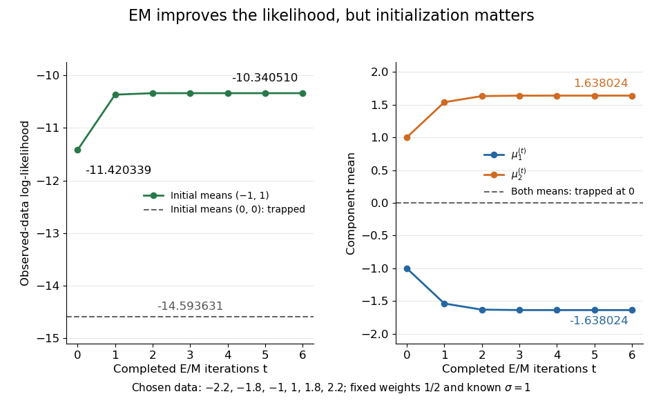
Likelihood ascent and mean updates for the chosen data, compared with an identical-means initialization
. Iteration zero is the initial fit; each subsequent point follows one E-step and one M-step. Starting at minus one and one increases the likelihood. Starting both means at zero leaves them at zero with a lower constant likelihood. All runs keep variance one and weights one half. Details.
For stable numerical evaluation, put and . The log-sum-exp function givesSubtracting keeps at least one exponential equal to one, avoiding the all-zero sum that direct evaluation of tiny component densities can produce.
In the Known-variance Gaussian mixture EM example, initialize both means at the same value . The mixture responsibilities are then for every observation. Each M-step sets both means to the sample mean, zero here; the next E-step again gives . Thus is a fixed point with log-likelihood , despite the better fit found from .
One can check the failure without trusting an iteration plot. Separate the means as and use the hyperbolic cosine identity:The Taylor expansion uses . Small nonzero separation therefore improves the log-likelihood, whereas translating both means to changes it by . This stationary point has both improving and worsening directions. Identical initialization cannot discover the separation because every observation keeps identical label probabilities. Trying several distinct initial fits and comparing their final log-likelihoods is useful, but does not prove global optimality.
Keeping the variance fixed also removes a different pathology. With known , every component probability density function is at most , so . If separate component variances are allowed to shrink without restriction, one mixture component can concentrate at an observation while another retains positive density at the other observations, making the likelihood function unbounded. The fixed positive variance in this example prevents that collapse; it does not remove initialization traps.
Articles by others on the same topic
There are currently no matching articles.