 Lagrange multiplier for quadratic cost

Suppose two adjustable inputs must deliver a prescribed total $c$, and their combined cost is the quadratic form $f(x,y)=x^2+2y^2$. These are chosen, dimensionless quantities; the coefficient $2$ makes concentrating an input in $y$ more expensive. Initially allow all real numbers $x,y$, with the equality optimization constraint $g(x,y)=x+y=c$. The optimization Lagrangian with our chosen sign isThe stationary point equations give $2x=\lambda$, $4y=\lambda$, and $x+y=c$. ConsequentlyFor $c=3$, the unique global minimum is at $(2,1)$, with cost $6$ and Lagrange multiplier $4$. Equal allocation would cost $6.75$; assigning everything to $x$ would cost $9$. At the optimum, the two marginal costs agree: ${\partial }_{x}f={\partial }_{y}f=4$. Moving a little input from one component to the other therefore has zero first-order effect on cost. When $c>0$, this solution also meets the extra nonnegativity optimization constraints $x,y\ge 0$, so it remains optimal with those added.

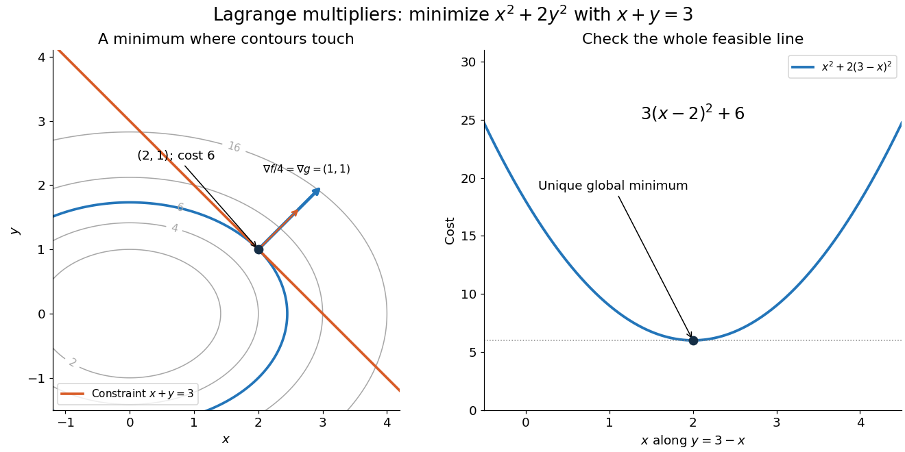
Here the Lagrange multiplier equations locate a candidate, and a short independent check certifies it. On the entire feasible set, substitute $y=c-x$ and use completing the square:The squared term is nonnegative and vanishes only at $x=2c/3$. Thus the candidate is the unique global minimum; there is no global maximum on this unbounded feasible set, a line. This separates finding a stationary point from proving optimality. The geometric beauty is that equal marginal costs, parallel gradients, tangency of level sets, and completing the square identify the same allocation.