
The matrix rank of an matrix over a field is the dimension of its column space, equivalently the dimension of its row space. It counts linearly independent column directions, with . Counting nonzero matrix entries gives a different quantity: an all-ones matrix can have arbitrarily many nonzero matrix entries and still have matrix rank one.[ref]
The Rank Theorem. Interactive Linear Algebra, §2.9, Definition: rank is column-space dimension; the row-space equality is proved below
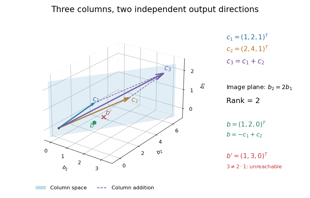
Consider the following matrix over the real numbers, with columns written as vectors:The vectors are linearly independent: requires both and , so . The third column adds no new direction to their linear span, hence despite all nine matrix entries being nonzero. The second row likewise repeats twice the first row.
The column space is a plane through the origin:Every output has second coordinate twice its first coordinate. Conversely, any vector equals , so this condition describes the entire plane, not just part of it. For example, is attainable, whereas lies outside the plane.

Elementary row operations expose the same count algebraically. Apply and , interchange the last two rows, multiply the second row by , and subtract twice the second row from the first. The resulting reduced row echelon form isThere are two pivot columns, so the matrix rank is two. The corresponding original columns form a basis of the original column space. The pivot columns of itself span the different plane with third coordinate zero: row operations preserve column linear relations, but generally move the column space.[ref]
Row Reduction. Interactive Linear Algebra, §1.2.2, Echelon Forms; §1.2.3, definitions of pivot position and pivot column
Solving the homogeneous linear system gives and . Taking the free variable givesThe kernel is the input direction that trades one unit of each of the first two columns for one unit of the third. This trade leaves the output unchanged. The rank-nullity theorem expresses the general balance: for an matrix of matrix rank , the nullity is . The column space describes reachable outputs; the kernel describes invisible changes to inputs.[ref]
The Rank Theorem. Interactive Linear Algebra, §2.9, Rank Theorem: rank plus nullity equals the number of columns
For the attainable output , one solution is . Every solution lies in the affine solution space of a linear equationIndeed, and . Conversely, subtracting from any solution gives a vector in the kernel, so this describes every solution. For , the same row operations on the augmented matrix expose : the second requirement demands where twice the first requires .
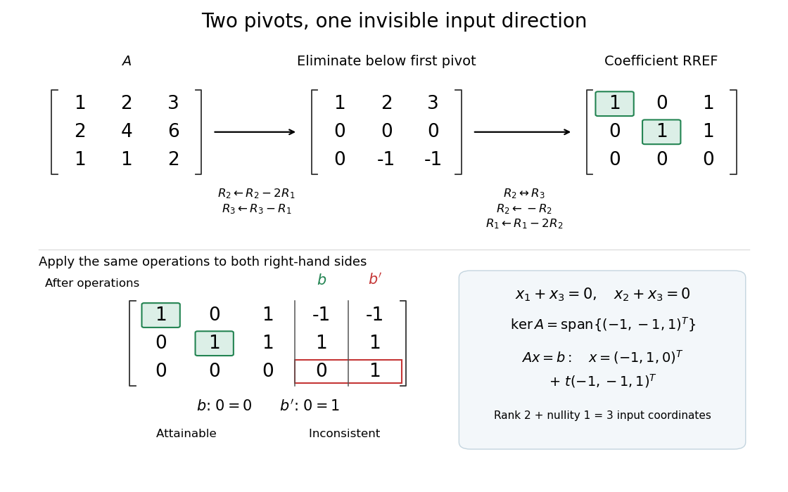
Two pivot columns, one kernel direction, and the same row operations distinguishing attainable from impossible
. Details. 
In general, a linear system is solvable exactly when appending leaves the matrix rank unchanged:Appending a vector outside the column space adds an independent direction. When a solution exists, every solution is , because . Thus one count predicts both how many output directions are reachable and, through the rank-nullity theorem, how many independent input directions remain free.[ref]
Solution Sets. Interactive Linear Algebra, §2.4.2, Key Observation and its proof; §2.4.3, Solution Sets and Column Spans
New to topics? Read the docs here!