 Solution

Balances and meanings. The first equation is conservation of energy per unit area. Here $c$ is effective areal heat capacity, $Q$ is the solar constant, and $Q/4$ accounts for the ratio of the Earth's intercepting disc area to its total surface area. The albedo $a$ reflects a fraction of that input. The outgoing thermal radiation is the Stefan–Boltzmann law modified by $\gamma (p)$, an effective transmission factor for the greenhouse effect; it normally decreases as atmospheric carbon dioxide increases.

The albedo relaxes towards its temperature-dependent equilibrium on the ice-adjustment time $t_i$. The atmospheric mass inventory per unit pressure is $M_{{\mathrm{CO}}_2}A/(M_{a}g)$, using the molar mass ratio of carbon dioxide to air and hydrostatic atmospheric mass. Its sources and sinks are volcanic input $v$, removal by chemical weathering over land area $A_L$ at rate $W$, and the atmosphere-to-ocean exchange $h(p-p_s)$. The ocean equation is a molar mass conservation balance: ${\rho }_{{\mathrm{H}}_2\mathrm{O}}{V}_{\mathrm{oc}}$ is ocean water mass, division by $M_{{\mathrm{CO}}_2}$ converts the incoming carbon-dioxide mass to moles, and $bC$ removes dissolved carbon by burial/export. With $C$ in moles per kilogram, $b$ has units of kilograms of water-equivalent per year.

Times and reduction. Linearize the temperature equation at fixed $a,p$ about radiative equilibrium. Its exponential relaxation time isThe equality uses $\sigma \gamma T^4=Q(1-a)/4$. A stock-over-flux thermal time, sometimes used as a scale, is four times this, $0.381\mathrm{y}$; both describe a rapid thermal response relative to the other processes.

For pressure in atmospheres, write $I=M_{{\mathrm{CO}}_2}A10^5/(M_{a}g)$ for the atmospheric carbon-dioxide mass per atmosphere. The factor $10^5$ is essential because $h$ is given per atmosphere. The pressure and slow ocean exponential relaxation times areThus $t_T\ll t_p\ll t_i=10^4\mathrm{y}<t_C$. The leading quasi-steady approximation givesSubstitution in the two remaining equations yieldsThe coefficient of $\dot{a}$ remains $t_i$; the printed $t_T$ in the reduced equation is a typographical error. Eliminating a fast temperature variable does not replace the ice-response time. The ocean time here is the slow time after atmospheric balance cancels the exchange flux; holding pressure fixed after imposing a carbon-dependent $p_s$ would describe a different conditional relaxation.

The supplied volcanic input givesabout $41.1\%$ of the stated present value $2.0\times 10^{-3}$; that value is about $2.43C_0$.

Carbon-dioxide levels. Since $A_{L}W=3.0\times 10^{11}\mathrm{kg}{\mathrm{y}}^{-1}=v$, the atmospheric balance with $p_s=C/K$ givesThis uses the specified present ocean concentration, as requested, rather than replacing it by the model's smaller volcanic-only equilibrium.

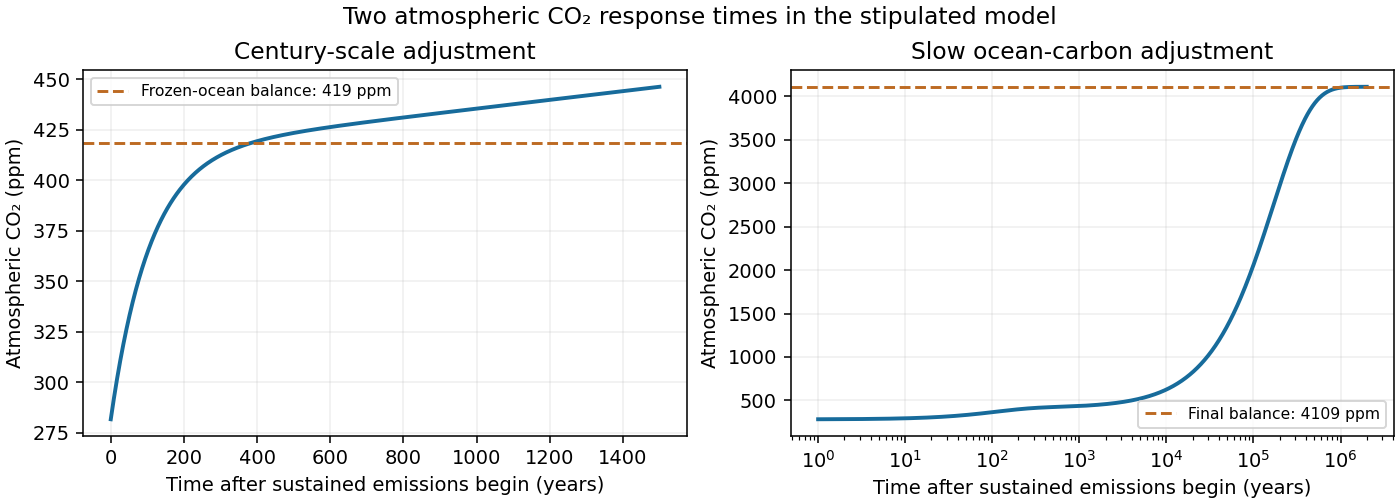
After sustained additional input $v_i$, $C$ barely changes during the atmospheric adjustment. At this stageThis is an intermediate balance, approached over several centuries. On the slower ocean time,with pressure following $p\simeq C/K+v_i/h$. Since $C(0)<C_{\infty }$, pressure continues to rise slowly. Its eventual level in this stipulated constant-parameter model isThe two-reservoir carbon adjustment therefore has a rapid rise towards the frozen-ocean balance followed by a much longer increase. The figure solves the coupled linear pressure–ocean equations, retaining their small inventory correction to the reduced time scales.