Polarization CHSH count model
ID: polarization-chsh-count-model

Let be orthogonal linear polarizations, and prepare the Bell state . The analyzer vector is ; its orthogonal companion has outcome . Direct inner products with the Bell state give and . Thus the expectation value of the outcome product is . These are physical polarizer angles; their corresponding Bloch sphere angles are doubled.
For a stipulated isotropic admixture, use the density matrixThe maximally mixed state contributes zero correlation, so for . Each local marginal is , independently of the other setting, illustrating quantum no-signalling. In this model is the interferometric visibility of the coincidence fringe; other noise models need not have one common visibility for every basis.
Choose , , and . The four correlations in the displayed CHSH inequality are . Consequently , exceeding the local bound exactly when . Perfect correlation at a single common setting would not yield this comparison between incompatible measurement in quantum measurements.
To connect probabilities with expected counts, stipulate emitted pairs per setting pair and independent detection efficiencies , independent also of settings, outcomes and hidden variables. The expected joint counts are . Their normalized correlation isFor original teaching inputs , , and , the expected counts are and . They total and give , hence . Fractional expected counts are not measured data. Efficiency cancels here because the loss model was specified to be independent; this algebra supplies no justification for discarding failures in an arbitrary Bell test with a detection loophole.
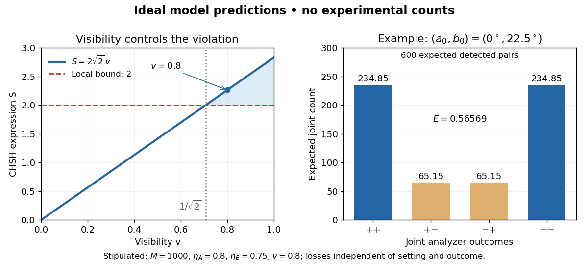
Ideal CHSH visibility threshold and expected detection counts
. Original model predictions, not experimental data. The first panel shows the visibility needed to exceed the local bound. The second uses 1000 emitted pairs, efficiencies 0.8 and 0.75, and visibility 0.8; each bar is an expected joint count. Details.
New to topics? Read the docs here!