 Sequential Bayesian photon counting

Consider an original balanced-readout model, rather than a fit to the experiment. Let $n\in \{0,\dots ,N_{\max }\}$, with a normalized prior probability $p_0(n)\ge 0$ and ${\sum }_n{p}_0(n)=1$. A detected chemical atom has outcome $s\in \{e,g\}$. Define the conditional probabilitiesHere $\chi$ is the accumulated quantum phase per photon, $\varphi$ the controlled analysis quantum phase, and $C$ the fringe contrast. The two probabilities sum to one for every $n$. Actual calibration may also require an offset and asymmetric detection errors; $C$ alone does not specify a quantum instrument.

Assume no photon number change during the record and fresh independently prepared atomic meters. For observed outcomes $s_1,\dots ,s_k$ at recorded settings ${\varphi }_1,\dots ,{\varphi }_k$, the Born rule and Bayes' theorem giveThe posterior probability is defined only for $Z_k>0$. Summing its numerator over $n$ proves normalization. This is also the update of diagonal elements of a field density operator under a measurement in quantum mechanics; it does not assume that an initial quantum superposition was an unknown pre-existing integer. The observed settings are part of the record, especially when selected adaptively.

For an exact finite example take $p_0=(1,1,1,1)/4$, $C=4/5$, and $\chi =\pi /2$. An $e$ outcome at $\varphi =0$ has likelihood $(9,5,1,5)/10$, giving $p_1=(9,5,1,5)/20$. Another $e$ at $\varphi =-\pi /2$ gives $p_2=(9,9,1,1)/20$. A subsequent $g$ at $\varphi =0$ givesThus three atomic records raise the posterior probability of $n=1$ from $1/4$ to $45/68$, while leaving finite uncertainty. No one of these outcomes identifies $n$ with certainty.

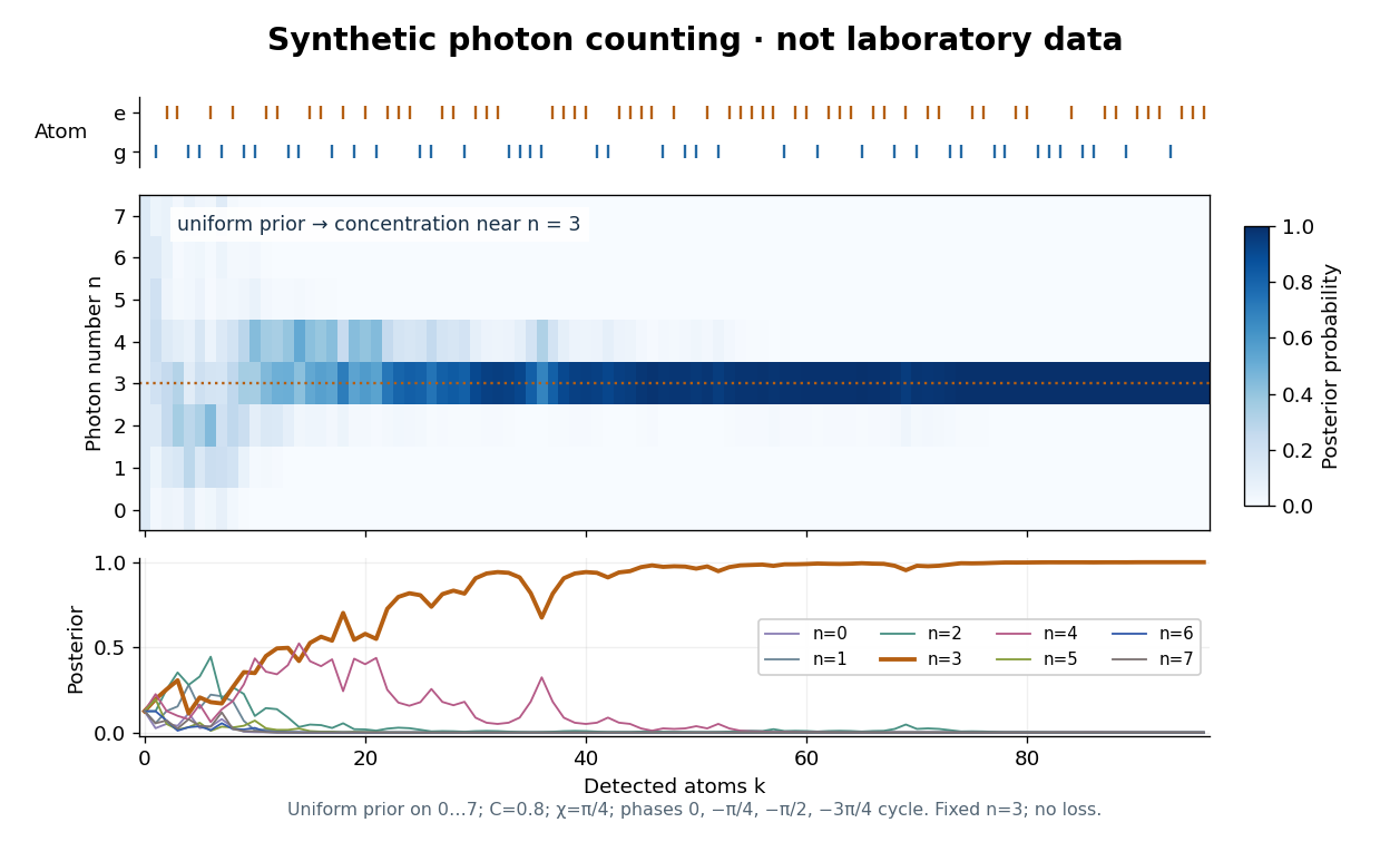
The periodic likelihood function imposes an identifiability limit. If $\chi =2\pi /q$ for an integer $q>0$, then $L_s(n+q;\varphi )=L_s(n;\varphi )$ for every setting: the posterior odds between $n$ and $n+q$ never change. Varying $\varphi$ can resolve a cosine reflection ambiguity within a period, but cannot remove this exact period. Changing $\chi$ can supply additional information. A finite cutoff is therefore a physical assumption to justify, not evidence that excluded high photon numbers were absent. At $C=0$ no outcome changes the prior probability; at $0<C<1$ neither binary outcome has an exactly zero likelihood.

The no-loss assumption also has a time limit. In an original zero-temperature loss model, let $\kappa =1/T_c$. A Fock state $|n⟩$ loses its first photon at rate $n\kappa$, so its survival probability is $\exp (-n\kappa t)$ and its mean lifetime is $T_c/n$ for $n>0$. Several records must be acquired within that lifetime to identify a plateau. When losses matter, first predict $p_k^{-}(n)={\sum }_m{T}_{nm}(\Delta t)p_{k-1}(m)$ using a normalized transition matrix, then apply the atomic Bayesian inference update to $p_k^{-}$. Thermal excitation requires upward transitions too. A delayed or broadened inference after a jump need not indicate that an atom caused the jump.