Bayesian statistics expresses uncertainty about an unknown statistical parameter through a probability distribution, then uses Bayes' theorem to update it after observing data. The prior distribution describes uncertainty before the current observations; the likelihood function describes how the statistical model generates those observations at each parameter value; the posterior distribution describes uncertainty conditional on the observations and that model. A physical parameter can have one fixed value while its value remains uncertain to us. Assigning it a probability distribution represents that uncertainty under the chosen model, rather than requiring the physical parameter to change randomly between measurements.
For example, suppose ten Bernoulli trials are independent conditional on an unknown heads probability , with a beta distribution prior . Eight heads and two tails give the posterior distribution by Beta-binomial conjugacy. Its posterior mean is , between the prior mean and observed binomial proportion . The Bayesian posterior below computes the whole update, and the credible interval below summarizes its remaining uncertainty. The conjugate update is explained in MIT 18.05, Reading 15: beta and normal conjugate priors.
The useful feature is that one posterior distribution supports several questions: a posterior mean estimates a value, a credible interval reports a range, and a posterior predictive distribution predicts a future observation while averaging over parameter uncertainty. With conditionally independent new data, today's posterior distribution can become tomorrow's prior distribution. These conclusions remain conditional on the statistical model and prior distribution; a precise update does not establish that either assumption fits the experiment.
A historical starting point is Thomas Bayes's essay in the 1763 volume of the Royal Society's Philosophical Transactions, communicated after his death by Richard Price. Its opening problem asks for uncertainty about an unknown event probability given observed successes and failures: the same direction of reasoning illustrated by the coin example. See Bayes and Price, An Essay towards solving a Problem in the Doctrine of Chances, opening letter and problem.
A credible set is a measurable set of parameter values containing specified posterior probability. At credibility level , it satisfies for a continuous posterior. A credible interval is a credible set that is an interval. Equal-tailed and highest-density choices add selection rules; the posterior-mass requirement alone does not make the set unique. Its probability statement is conditional on the observed data and prior model, whereas a frequentist confidence interval is interpreted through repeated-sample coverage.
If inclusion depends only on fully observed data , then cancels from Bayes' theorem for that individual's parameters. Selection can still matter for unknown population parameters and for missing or unconditioned features. For independent detected observations conditional on their count and population parameters , each likelihood has normalization . A model for the detected count adds its own count likelihood. Do not combine a selected-population prior with a truncated-data likelihood in a way that counts the same selection twice.
For data , a positive prior distribution density and likelihood function , Bayes' theorem gives posterior density . Thus reconstructs the likelihood up to a constant. Estimate the posterior density from simulation, divide by the known prior density and maximize over the search region. A posterior mode alone instead estimates a maximum a posteriori estimate; it estimates a likelihood maximizer only when the prior is constant there. Prior support must include the likelihood maximizer of interest.
// Target: biology.bigb
BUGS specifies a probabilistic model through stochastic nodes, deterministic nodes and observed data, then uses Markov chain Monte Carlo to simulate its Bayesian posterior. Its normal sampling notation uses a precision parameter rather than a variance, and its gamma notation uses shape and rate.
A zeros trick implements a positive likelihood function by adding an observed zero with Poisson distribution mean . If this mean is nonnegative throughout the parameter support, its likelihood is and yields the intended Bayesian posterior. The constant must be independent of the parameter; arbitrary clipping changes the target.
Variational inference approximates a posterior distribution by minimizing a Kullback-Leibler divergence over a chosen family of probability distributions. For an unnormalized posterior density and a trial probability density function , minimizing is equivalent to minimizing .
The variational approximation gap is the part of the evidence lower bound deficit that remains even after optimizing separately for an observation within a specified variational family. With the generative model fixed and finite , defineThe equality uses the usual evidence lower bound identity for variational inference. A supremum allows for a best value that is not attained. The amortization gap separately measures failure of the shared inference rule to reach this value.[ref]
Inference Suboptimality in Variational Autoencoders by Chris Cremer and others. Table1; §3.1, equation8, decomposition for the ordinary variational-autoencoder bound
An original example shows what independence can cost. Stipulate a centred two-dimensional multivariate normal distribution as the posterior distribution, with covariance matrixRestrict the variational family to centred independent normal distributions, with . This is a simple mean-field variational inference restriction. Writing , the Kullback-Leibler divergence between normal distributions becomesEach variance contributes a term , minimized at . ConsequentlyFor , the best independent variances are both , and the unavoidable deficit is about nat. Matching both marginal variances to one instead would give about nat. The reverse Kullback-Leibler divergence therefore chooses narrower independent marginals here, while still failing to represent the correlation.
Enlarging the family to include the full covariance matrix permits and reduces this example's gap to zero. More generally, inclusion cannot increase the optimum approximation gap at a fixed model. Merely training the same shared rule longer cannot remove a strictly positive family restriction. Numerical improvements are not proofs that the infimum has been reached.
A normalizing flow constructs a probability distribution by passing a simple reference random variable through invertible differentiable transformations. The change of variables formula supplies its probability density function: if and is a diffeomorphism between equal-dimensional spaces, thenThe Jacobian determinant accounts for local expansion or contraction of volume. Composing several transformations gives a flexible distribution while retaining a computable density, useful for a richer approximate posterior distribution in variational inference.[ref]
Variational Inference with Normalizing Flows by Danilo Jimenez Rezende and Shakir Mohamed. §3, equations5–7, invertible transformations and composition
For an original nonlinear example, let have the standard normal distribution with density , and set . Since and tends to opposite infinities at the two ends of the real line, every output has exactly one preimage. Its probability density function satisfiesAt , the output is and . The factor reflects how strongly the transformation stretches nearby inputs. Integrating after the substitution cancels this factor against , leaving total probability one.
For , the chain rule givesGenerating transformed samples alone does not evaluate their probability density function; evaluating the determinant factors is essential. The single-preimage formula also requires invertibility: the map folds two real inputs together, so it cannot be substituted into this formula unchanged.
Amortized inference learns one shared rule that maps observations to approximate posterior distributions, spreading the work of fitting that rule across many inputs. Instead of separately optimizing variational parameters for every observation , a recognition network returns the parameters of . The shared parameters are learned across data; evaluating the rule for a new input is then a different operation from fitting it.[ref]
Stochastic Backpropagation and Approximate Inference in Deep Generative Models by Danilo Jimenez Rezende and others. §4, recognition model and joint optimization
A scalar Gaussian model gives an exact example. Let and . Completing the square givesThe shared rule , with , and fixed variance , represents the exact posterior for every real . Evaluating replaces a separate optimization for each observation in this stipulated model. It does not imply that every nonlinear latent-variable model has an exact rule this simple.
Sharing can introduce an additional restriction even when the chosen distribution family is adequate. For observations and , the exact posterior means are and . The Gaussian family can represent each exactly when is fitted separately. If the shared rule is constrained to output one constant mean for both inputs, its best equal-weight choice is . Each case then hasThis original example isolates an amortization gap: the loss from restricting how observation-specific variational parameters are produced, rather than an inability of the per-observation Gaussian family to express the target. The shared mapping's capacity and its training therefore matter alongside the family of probability distributions.
The amortization gap measures how much evidence lower bound is lost by using the distribution returned by amortized inference instead of the best distribution available for that observation in the same variational family. Hold the generative parameters fixed. Write for the evidence lower bound and suppose the optimum is attained. For the shared rule ,The remaining variational approximation gap is , so the total loss isThus a restrictive recognition network or incomplete training can leave an amortization gap even when the variational family can represent the exact posterior distribution.[ref]
Inference Suboptimality in Variational Autoencoders by Chris Cremer and others. Table1, summary of gap terms; introductory definition of the optimal approximation within its family
For an original example, stipulate for equally weighted observations and . The variational family represents both posterior distributions exactly when fitted separately, so . Restrict the shared rule to : it can adjust the intercept but its slope is fixed at one. The Kullback-Leibler divergence between these unit-variance normal distributions is . Averaging the amortization gap over the two observations givesThe best shared intercept still loses nat on average. A current rule with loses one nat: half a nat can be removed by training this rule better, while the remaining half requires changing its fixed-slope restriction. This separates the variational family's expressive power from the shared mapping's capacity and current training state.
In a numerical comparison, a locally improved per-observation distribution need not be the global optimum . Its improvement supplies a lower bound on the true amortization gap; failing to find an improvement does not establish a zero gap. Comparisons must keep both and fixed.
Under fixed-support regularity permitting differentiation under the integral sign, apply the product rule to . The first derivative term is and the second is . This proves the displayed identity. For an evidence lower bound, take , holding noise fixed in the inner derivatives. Parameter-independent continuous noise contributes a reparameterization gradient; untransformed discrete choices contribute a score-function gradient estimator. A mixed base law cannot be called parameter independent if its discrete factors retain variational parameters.[ref]
A guide program is a probabilistic program whose generated probability distribution approximates a model's posterior distribution. Its adjustable parameters are fitted by variational inference. The guide must assign probability only where the target allows it when minimizing , but a tractable guide can still miss important target regions.
A reparameterization gradient differentiates an expected value by representing the simulated random variable as a differentiable transformation of parameter-independent noise. For , the identity requires justified differentiation under the integral sign. For a normal distribution, use with drawn from the standard normal distribution.
Gaussian reparameterization represents a random variable with a normal distribution using a location, a scale and parameter-independent noise:Here has the standard normal distribution. The resulting has expected value and variance . The probability distribution is unchanged; the representation separates the random draw from the adjustable parameters. This makes reparameterization gradients available for differentiable expectations, including the Gaussian approximate posterior in a variational autoencoder.[ref]
Stochastic Backpropagation and Approximate Inference in Deep Generative Models by Danilo Jimenez Rezende and others. §3.2, Gaussian location-scale transformation and equation(10)
For a complete example, fix and considerHolding the same noise value fixed while differentiating givesAt , , the particular noise draw gives and derivative estimate , while the true derivative is . An individual sample need not equal the derivative; the equality is in expected value.
Parameterizing a positive scale as also gives . One can differentiate through the deterministic transformation while leaving the noise law fixed. For a general integrand, exchanging derivative and expectation still requires justified differentiation under the integral sign; the representation alone is not a proof of that exchange. Reusing noise when parameters change also connects the construction to common random numbers.
Consider the explicitly specified objectiveand estimate its derivative by a symmetric finite difference with step . The choice of shared or independent noise changes the estimator's variance even though both use correct normal distributions at the two parameter values.
With common random numbers, the same appears on both sides:Thus and , independent of . Cancellation removes the noisy square term. For this quadratic, the symmetric difference has no truncation bias in exact arithmetic.
For independent standard normals , instead useIf , expand . The standard-normal moments , and giveAdding the two independent square variances and dividing by yieldsBoth estimators have the correct expected value , but the independent-noise variance diverges as tends to zero. At and , the variances are and . An average of independent replicate estimators divides each variance by .
This is a complete calculation for the stated quadratic, not a universal dominance theorem. At , and , the independent variance is , below the shared value . The covariance principle in common random numbers explains why coupling needs a specified objective and comparison. Very small steps in floating-point evaluation also introduce cancellation concerns that this exact-arithmetic model does not include.
Markov chain variational inference optimizes an initial parametric probability distribution by minimizing after a fixed number of Markov kernel updates. The best initial probability distribution can depend on ; Kullback-Leibler divergence contraction does not imply that optimization commutes with applying the Markov kernel.
Mean-field variational inference restricts the trial probability density function to . With the other factors fixed, , provided this expression has a finite positive normalization constant. Subtracting the objective at leaves , proving the update is optimal when the terms are well defined.
Data augmentation enlarges a posterior distribution with latent variables whose removal by marginalization recovers the original posterior distribution. Convenient full conditional distributions then permit a Gibbs sampler on the enlarged space.
A hierarchical Bayesian model assigns distributions to local latent variables conditional on shared hyperparameters, then distributions to observations conditional on those latent variables. Its probabilistic graphical model records this conditional factorization, often using a plate for repeated observations. Integrating out latent variables gives the marginal likelihood of the hyperparameters. Priors described as flat on logarithms require a Jacobian determinant when densities are written in the original positive variables.
Unknown hospital event probabilities can be modelled as exchangeable random variables conditional on shared hyperparameters, for example independently. Different sample sizes affect the binomial observations but do not by themselves invalidate exchangeability of the risks. Known systematic covariate differences, such as case mix or procedure type, should instead enter the risk model; only residual effects may then be exchangeable. Exchangeability permits heterogeneous realized risks and is not an assertion that all risks are equal.
// Target: biology.bigb
A normal local effect can be represented by a standardized latent variable independent of the hyperparameters, with . This preserves the hierarchical model while changing the coordinates explored by Markov chain Monte Carlo. It often improves mixing when individual effects are weakly informed, reducing strong scale-effect dependence. Centered coordinates can be better with very informative individual data. The stochastic prior on implements the transformation correctly; re-expressing an existing density directly instead requires the appropriate Jacobian determinant.
Partial pooling estimates related local parameters jointly through shared hyperparameters. Each local Bayesian posterior balances its own likelihood function against a group prior distribution, with stronger shrinkage when its data are weak or the group variation is small. It lies between forcing all local parameters to be equal and estimating them independently. Random-effects meta-analysis is an important application.
A Gamma–Poisson hierarchical model uses , , and , with gamma distributions in shape-rate convention. Conditional independence gives full conditional distributions and .
For and , a scale-invariant prior induces the Haldane prior on . Integrating out each local mean gives . Thus for . The gamma full conditional distribution has mean , so the tower property gives , equal to the displayed partial pooling formula. For , the posterior is improper and this expectation is undefined.
For independent Poisson distributions with means and a shape–rate Gamma distribution prior on , integrating adds to the total-count exponent and to the sum of relative rates. This distinguishes gamma mixing from conditioning on the total count, which gives a multinomial distribution.
An observed astronomical colour is the sum of a normal intrinsic colour, a nonnegative dust contribution with an exponential distribution, and normal measurement noise. With latent , and , the Gibbs sampler conditionals for are normal and those for are truncated normal distributions. A flat prior on and inverse-gamma priors on give inverse-gamma conditional updates for the two scales. Log-flat priors on both scales instead make the joint posterior improper when all , despite formally proper full conditionals at generic latent states: the marginal observed likelihood has a positive limit at either zero-scale boundary. Proper positive-scale priors restore a genuine joint posterior.
Maximum a posteriori estimation selects a parameter value maximizing its posterior density relative to a specified reference measure. Its output is a maximum a posteriori estimate. The maximizing value need not be invariant under a nonlinear reparameterization, because a density transforms with a Jacobian.
A maximum a posteriori estimate maximizes the posterior density of a parameter or latent configuration. Equivalently, it maximizes the sum of the log likelihood and log prior, relative to the chosen reference measure.
A credible interval is an interval containing a prescribed amount of posterior probability for an unknown scalar statistical parameter . For a continuous posterior distribution with posterior density , its endpoints satisfyThe conditioning includes the chosen statistical model and prior distribution. For a discrete posterior distribution, exact equality may be impossible because of its probability masses; an interval can instead be required to contain at least the requested posterior probability. An interval compresses the full posterior distribution into a range whose uncertainty can be communicated in the parameter's own units. See MIT 18.05, Class 16: probability intervals.
For the eight-head, two-tail example in Bayesian statistics, the posterior density is on . Its cumulative distribution function, obtained by integration of this polynomial, isSolving and by the bisection method givesThese are numerical approximations to the exact quantiles defined by those equations; the endpoints were computed from the cumulative distribution function, rather than read off a plot. The resulting equal-tailed credible interval leaves 2.5% posterior probability on each side. Its shaded area is 95% of the total area under the posterior density.
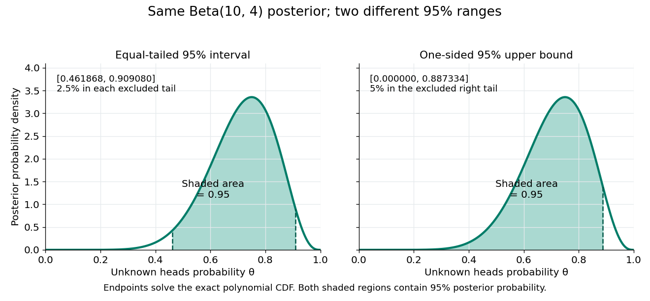
Credible intervals are not unique. The one-sided credible interval also has 95% posterior probability, but leaves all 5% outside it on the right. A highest density region instead selects points above a density threshold; it need not be an equal-tailed credible interval, and when the posterior density has separated peaks it need not be one interval at all. Thus a reported credible interval should specify its construction.
A 95% credible interval makes a statement about the statistical parameter conditional on these observed data and the Bayesian model. A 95% confidence interval instead refers to the coverage probability of a procedure under repeated sampling at a fixed parameter value. These are different conditioning statements: 95% posterior probability does not by itself imply 95% coverage probability for every fixed parameter. The confidence interval article develops that sampling interpretation.
A highest posterior density interval is a credible interval whose included points have at least as high posterior density as excluded points, apart from boundary and null-set choices. It is a highest density region of prescribed posterior probability that happens to be an interval. For a continuous unimodal posterior with two interior endpoints, the endpoint densities agree. A monotone posterior on a half-line instead starts at a support boundary, as in a Pareto highest density interval. For a multimodal posterior distribution, the highest-density region can be disconnected and cannot always be represented by a single interval. Density-level regions use a specified parameter coordinate and reference measure; they are not generally preserved by nonlinear reparametrization.
For a beta distribution with shape parameters , the probability density function vanishes at zero and one and is strictly increasing up to and strictly decreasing afterwards. This follows because the derivative of its logarithm is , whose sign changes at .
For each , the highest posterior density interval when this beta distribution is a posterior distribution has unique endpoints determined byThe second equation gives equal endpoint posterior densities. For every density threshold strictly between zero and the modal height there is precisely one crossing on each side. The enclosed probability is continuous and strictly decreasing from one to zero as the threshold increases, proving existence, uniqueness and the highest posterior density interval property. The restrictions are essential to this two-interior-endpoint characterization; monotone cases use a support boundary instead.
An equal-tailed credible interval uses quantiles of a continuous posterior distribution to leave posterior probability in each tail. It is also called a central credible interval; central refers to equal tail probabilities, not equal distances from the posterior mean. For the beta distribution in credible interval, the 95% endpoints are approximately and , whose midpoint differs from the posterior mean .
A one-sided credible interval puts all excluded posterior probability in one tail. For a continuous posterior distribution, an upper bound satisfies ; a lower bound uses . Intersecting with the parameter's allowed range removes points of zero posterior probability. For the beta distribution , the upper 95% bound is , so is the alternative credible interval shown above.
An empirical Bayes method estimates prior hyperparameters from the marginal distribution of the observed data and then uses the resulting fitted prior in Bayesian inference.
A maximum marginal likelihood estimator chooses a hyperparameter by maximizing the data density obtained after integrating the model parameter against its prior distribution.
A hyperparameter controls a family of prior distributions or statistical models and is fixed, estimated, or assigned a further prior at a higher level of a hierarchical model.
A hyperprior is a prior distribution assigned to a hyperparameter that controls another prior distribution. In a hierarchical Bayesian model, this makes uncertainty about the prior's parameters part of the joint probability model, rather than replacing those parameters by fixed numbers.[ref]
Stan User's Guide by Stan Development Team. Version2.37, Regression Models, Hierarchical priors
For data , a model parameter and a hyperparameter , a common factorization isHere supplies the likelihood function, is the conditional prior distribution, and is the hyperprior. After observing , Bayesian inference gives a joint posterior distribution. The marginal posterior of averages over the updated hyperparameter distribution:For discrete hyperparameters, the integral is replaced by a sum.
An exact example makes the averaging visible. Let be a success probability and choose a two-point hyperprior,Both conditional beta distributions have expectation , but they concentrate differently around it. Now observe two successes that are independent conditional on , each with a Bernoulli distribution. Their conditional probability is . Integrating against the two possible priors givesThus the data also update the hyperparameter:The conditional posterior distributions of are respectively and . Their posterior mixture has meanThis is an original illustrative probability model, rather than data or a numerical example from the guide.
Fixing at its prior mean would instead produce after the same observations, with posterior mean . Averaging the hyperparameter first has changed the model; it does not reproduce averaging the conditional posteriors with their updated probabilities. A hyperprior therefore adds a specified layer of uncertainty, while its own choice remains part of the assumptions of the hierarchical Bayesian model.
A Dirichlet process is a probability distribution over probability measures. For concentration and base probability measure , write . Every finite measurable partition satisfieswith zero-base-mass cells assigned zero mass. Consequently and : larger concentration keeps random masses closer to the base measure.
For conditionally independent and identically distributed observations , the posterior isThis follows by Dirichlet-multinomial conjugacy on each partition. It supplies a tractable prior distribution for an unknown distribution without choosing a fixed-dimensional parameter family.[ref]
Draws are almost surely discrete on the usual standard Borel sample spaces, even when is continuous. A Dirichlet process prior on a mixing measure can still yield a continuous mixture density.
A Dirichlet prior with parameters combined with categorical labels having counts gives a Dirichlet posterior with parameters .
Prior probability describes uncertainty before the current observations are incorporated. For a statistical parameter , a prior distribution assigns probabilities to its possible ranges, conditional on background information and a statistical model. A continuous prior density specifies these probabilities through integration:Here the probability density function is relative to Lebesgue measure ; a discrete prior distribution instead uses a probability mass function and sums. Density at one point is not the probability of that point. A nonnegative kernel with infinite total mass is an improper prior, whose use requires a separate check of posterior propriety.
For the coin model in Bayesian statistics, the beta distribution has prior density on . Its mean is and its variance is . It favors moderate heads probabilities without ruling out values near zero or one. For example,The prior curve in Bayesian posterior makes this preference visible; moment matching for a beta prior explains how to choose a beta distribution from a desired mean and variance.
A prior distribution lets earlier evidence or elicited knowledge contribute to statistical inference when the current sample size is limited. It also exposes assumptions that can be checked by prior elicitation and a prior predictive check. Before the same eight heads and two tails, a uniform prior would give posterior mean , compared with under : the observations do not uniquely determine a Bayesian posterior. Even a uniform prior makes a choice of parameter coordinates; its child article explains why changing coordinates can destroy uniformity.
A class prevalence applicable before considering the current case-specific evidence. Under random sampling from the relevant reference population, it sets the prior class probability used in Bayes' theorem.
The prior mean is the expected value of a statistical parameter under its prior distribution, when this expected value exists. The posterior mean instead uses the posterior distribution after conditioning on observations.
Translate external information into a prior distribution by asking for representative values, uncertainty intervals and tail probabilities. Fit parameters of a suitable distribution to those judgments and inspect the resulting prior predictive distribution. For a probability believed near , a beta distribution with parameters has the desired mean; its concentration can be chosen to match a stated probability of exceeding . The words “near” and “unlikely” alone do not specify one unique prior.
For two exhaustive mutually exclusive models of positive prior probability, prior odds compare their probabilities before observing the data. They must be distinguished from the parameter prior distributions within those models. A Bayes factor multiplies these prior odds to produce posterior odds.
A prior density is the probability density function of a continuous prior distribution with respect to a specified reference measure. A proper prior density is nonnegative and integrates to one. Prior-density factors enter Bayesian posterior and RJ-MCMC acceptance formulas along with the likelihood and model prior probabilities.
A continuous spike-and-slab prior mixes a narrow continuous probability distribution around zero with a much wider component. It permits practical effect selection while retaining a continuous posterior density. Its narrow component is not the exact-zero mass of a point-null mixture prior. A latent component indicator aids computation; a wide-component draw can still have small magnitude, so posterior effect thresholds and component membership answer different questions.
A uniform prior on a finite-volume parameter region assigns constant probability density there and zero outside. On it is , giving a beta distribution posterior after binomial distribution data. Uniformity depends on the coordinate: a nonlinear reparametrization introduces a Jacobian and generally does not preserve a uniform density.
The Bayesian posterior is the conditional probability distribution of an unknown statistical parameter after observing data. Suppose a continuous prior distribution has prior density relative to Lebesgue measure , and is the sampling probability mass function or probability density function of the observed data in the statistical model. Bayes' theorem givesThe Bayesian model evidence is the normalization constant making the posterior density integrate to one. The strict positive, finite condition is essential: a zero or infinite normalizer does not define this posterior distribution, even if the unnormalized expression can be written down. Other reference measures give the corresponding density formula; discrete parameter values replace the integral by a sum. The posterior propriety article gives examples where normalization fails.
With fixed, is a likelihood function of . Its normalization as a sampling distribution is over possible data, not over parameter values. In particular, a likelihood function is not a probability density function for and need not integrate to one over . The prior density supplies the probability weighting, and the Bayesian model evidence normalizes their product. This distinction prevents a tempting mistake: reversing the conditioning merely by exchanging the words “data” and “parameter”.
For eight heads among ten conditionally independent Bernoulli trials, take the observed data to be the heads count . Its binomial distribution likelihood function and the prior density giveUsing the Euler beta function , the Bayesian model evidence and normalized posterior density areThus the posterior distribution is . If the data are instead one particular ordered sequence with eight heads and two tails, its likelihood function omits the factor 45 and its Bayesian model evidence becomes . The factor cancels in Bayes' theorem, leaving the same posterior distribution; these two data descriptions have different sampling probabilities but identical information about here.
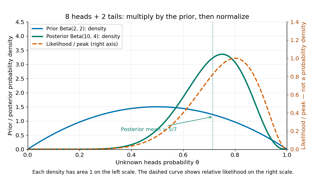
Beta(2,2) prior, peak-normalized Bernoulli likelihood, and Beta(10,4) posterior after eight heads and two tails
. Details. The prior density and posterior density use the left axis and each integrate to one. The dashed likelihood function uses the right axis and is divided by its maximum solely to compare its shape; it is not a parameter probability density function. The likelihood function peaks at , while the posterior mode is and the posterior mean is . Multiplying by the prior density shifts the preferred values toward one half while preserving a range of possibilities.
The resulting posterior variance is , compared with prior variance . In this example the update reduces uncertainty. The posterior predictive probability of heads on the next conditionally independent toss is , and the credible interval above reports a 95% range. These are summaries of the same posterior distribution, rather than competing estimates of one density peak.
For independent and identically distributed observations from a normal distribution with known variance , an exponential distribution prior of rate on their nonnegative mean gives this truncated normal distribution posterior. Complete the square in ; the truncation remains essential even when the untruncated normal mean is negative.
A posterior moment is a moment computed under a posterior distribution. Its first raw moment is the posterior mean; its second central moment is the posterior variance.
For one observation from a continuous uniform distribution on and prior density , the likelihood cancels the factor and leaves . Normalization gives posterior density , for . Its mean is and variance one. The Bayes estimator under squared error loss is therefore , unchanged by multiplying the loss by a positive constant.
For independent observations uniform on and a uniform prior on , the likelihood is constant wherever all data-compatible intervals overlap. The posterior is therefore uniform on the displayed intersection, provided it has positive length. Both squared-error and absolute-error Bayes estimates are its midpoint. An empty or zero-length interval has zero marginal likelihood and cannot be normalized into this ordinary posterior density.
For one uniformly sampled integer , the likelihood function for the unknown endpoint is . A flat improper prior on positive integers gives an improper posterior distribution, since the harmonic series diverges. A reciprocal prior instead gives a proper posterior proportional to for , with approximate survival probability and finite quantiles, but infinite posterior mean. A uniform prior cut off at gives posterior mean , demonstrating sensitivity to that arbitrary cutoff.
For continuously distributed uncertain quantities, define rank one to be the largest. A joint posterior distribution induces a discrete distribution on each quantity's rank. Estimate it by ranking the whole vector in each joint draw and averaging rank indicators; the probability of rank one is the probability of being largest. Ranking posterior means does not recover this uncertainty. The joint draws must preserve any posterior dependence, and tie conventions must be specified for models with atoms.
A posterior variance is the variance of a parameter under its Bayesian posterior, namely when finite. It describes remaining uncertainty after observing data and is distinct from the repeated-sampling variance of a fitted estimator.
For a vector parameter with finite second moments and posterior mean , the posterior covariance matrix records its uncertainty and linear dependence after conditioning on the observations. Its diagonal entries are posterior variances. In a regular locally flat-prior normal distribution approximation it is the inverse observed information. A quadratic form has posterior expectation equal to the form at the posterior mean plus the trace of its matrix times this covariance.
The distribution of a new or missing quantity integrates its model over the Bayesian posterior: . Both parameter and residual uncertainty should enter predictive draws used for multiple imputation.
If future Bernoulli random variables are conditionally independent given a shared parameter , with success probability , their all-success conditional probability is . Taking a posterior expectation proves the identity. For , Jensen's inequality and give . For two distinct future trials the posterior covariance is . Thus shared parameter uncertainty can induce positive dependence even when trials are conditionally independent.
A posterior predictive check compares a summary of the observed data with the same summary in replicated data drawn from a model's posterior predictive distribution. The replication must match the target: replicating an existing group's observations conditional on its effect differs from predicting a new group with a newly drawn effect. Such checks expose mismatches in dispersion, tails or other features; using the observations to fit and check the model means they are not automatically calibrated frequentist tests.
In a hierarchical Bayesian model, replication conditional on fitted observation-level random effects checks the sampling layer. Replication with fresh random effects drawn from their population law also checks the population mean and variation. To assess a dose-response curve, sample the global parameters from their posterior distribution, draw fresh effects for new plates at each existing dose, and compare replicated means, spreads and trend discrepancies with the observed values. Reusing the fitted plate effects can conceal a misspecified mean curve by reproducing deviations those effects already absorbed.
For independent observations , put , , , and . Integrating the likelihood function against a flat improper prior on gives, up to the arbitrary prior constant,Indeed , and the remaining one-dimensional Gaussian integral is . The conditional Bayesian posterior of is .
A posterior predictive probability averages a future-event probability over the Bayesian posterior. For a Bernoulli distribution with unknown parameter , it is . Under Beta-binomial conjugacy with posterior , the predictive success probability is .
A posterior density is the density of a posterior distribution with respect to a chosen reference measure.
The log-posterior is the logarithm of a positive posterior density. Its gradient is the posterior score control variate when boundary terms vanish. An additive constant independent of the parameter does not affect optimization or differentiation.
The posterior mean is the expected value of a parameter under its posterior distribution; under squared-error loss it is the Bayes estimator.
Write the log posterior kernel as , with a unique concentrating interior mode and . Apply Laplace's method to the numerator and denominator of the expected value under the posterior distribution. Their common leading Gaussian factor cancels. Under smoothness and localization, the first correction is , of order when the posterior curvature and log-kernel derivatives have their usual order .
A posterior probability is the probability assigned to an event by the posterior distribution after conditioning on the observed data.
For two exhaustive mutually exclusive models, posterior odds are the ratio of their posterior probabilities. Bayes' theorem givesThe second factor is the Bayes factor, formed from model prior predictive distributions. Evidence favouring one model need not make that model's posterior probability exceed one half if its prior probability was sufficiently small.
When the prior odds of a real effect are , a study's Type I error is , and its statistical power is , a positive report updates those odds to . This follows directly from Bayes' theorem. A small false-positive rate does not itself make the effect's posterior probability high: the prior odds and power also matter. The posterior exceeds one half exactly when .
A point-null mixture prior assigns positive mass to one parameter value and distributes the remaining mass continuously over alternatives. Posterior point mass is obtained by dividing the null component of the marginal density by the full marginal density.
Suppose independently, and compare with for fixed , using equal prior model probabilities. Put . The posterior probability of a Gaussian point null isHolding fixed while leaves the two-sided p-value unchanged but makes the null posterior probability tend to one. For , and , the p-value is about , while the null posterior is about .
The two procedures answer different model-based questions: a tail probability under the point null and a comparison of that null with a specified alternative prior distribution. The alternative's fixed prior scale spreads mass over parameter values much wider than the increasingly precise likelihood. This is the Jeffreys-Lindley phenomenon, not a conversion formula from p-values to posterior probabilities.[ref]
Bayes Factors by Robert E. Kass and Adrian E. Raftery. Section 5.2, discussion of sample size and point-null testing
An improper prior is a nonnegative prior kernel with infinite total mass. It can still produce a proper posterior after multiplication by the likelihood and normalization.
The Haldane prior has formal beta distribution parameters . It is an improper prior, with infinite mass at both endpoints of . For a binomial distribution likelihood with successes and failures, its posterior is only when . A density flat in the log odds induces this kernel by the Jacobian determinant .
The measure is invariant under multiplication by every positive constant. In the logarithmic coordinate it is Lebesgue measure. It cannot be normalized over , although a bounded truncation is a log-uniform distribution.
A random-effect model with positive marginal likelihood at scale zero cannot yield a proper posterior distribution under a prior proportional to the reciprocal scale near zero. On a compact set of the other parameters, continuity and positivity give a positive likelihood lower bound, while . Individual full conditional distributions can still be proper, so their existence alone does not justify a Gibbs sampler with a probability distribution as its joint target.
A posterior kernel defines a posterior distribution exactly when its integral is finite and nonzero. Proper full conditional densities do not suffice. For example, if a known positive measurement variance makes a marginal normal likelihood approach a strictly positive limit as a latent variance tends to zero, the log-flat prior gives infinite posterior mass at that boundary. The same problem occurs for a latent exponential scale with when the observed likelihood has a positive limit as the exponential contribution vanishes.
If a model configuration leaves a parameter absent from its likelihood function, giving that parameter an independent flat improper prior makes the posterior distribution normalization infinite whenever the configuration has positive prior distribution mass. Integrate first over that parameter: a positive constant likelihood function factor is repeated over all of . This occurs for the second segment mean of a Gaussian change-point detection model when the proposed split is after the final observation. There is no posterior distribution or valid Gibbs sampler for that joint kernel. A proper prior distribution on the unused parameter is necessary if the no-change configuration is retained.
For conditionally independent Poisson observations of mean and a gamma distribution prior of shape and rate , the likelihood function contributes . Multiplying by the prior density gives a posterior distribution with shape and rate . The single-observation update is shape and rate .
The posterior mean is the convex combinationThus the prior mean and the sample maximum-likelihood estimate bracket it. Integrating the next conditional Poisson distribution against this posterior distribution gives the Poisson-gamma mixture, a negative binomial distribution; its spread includes uncertainty in as well as the conditional count variation.
If the positive baseline rate has a gamma distribution of shape and rate , its logarithm has this probability density function with respect to . The extra factor is the Jacobian determinant of the transformation. After a Gibbs sampler draws the conditional baseline rate, taking its logarithm is an exact update of the intercept. Omitting the Jacobian changes the prior.
Given , independent observations have Poisson distribution with means for known exposures. A gamma distribution prior of shape and rate yields a gamma posterior with shape and rate . The likelihood kernel is . Thus the posterior mean depends on total claims and total exposure, not the number of periods alone.
A gamma prior with shape and rate combined with independent observations from an exponential distribution of rate gives the posteriorUnder squared-error loss, the Bayes estimator is its posterior mean .
With a uniform prior distribution on a Bernoulli chance , successes yield posterior density . Integration gives next-trial success probability , but the singleton retains probability zero. More generally, ordinary conditioning with a finite integrable likelihood and positive finite normalization constant preserves absolute continuity, so a continuous prior does not acquire a new atom at certainty from a finite sample.
For independent geometric random variables with success probability , observing terminal events and preceding failed Bernoulli trials gives likelihood function proportional to . Multiplication by a beta distribution prior gives the posterior distribution . With complete waiting times , take and .
A waiting time that is right-censored after failed trials contributes : increase by without increasing . This requires the censoring mechanism to be ignorable, as with an externally fixed observation horizon. Counting a censored waiting time as an observed event changes the likelihood function and biases the update.
Mix a binomial distribution with a beta distribution for its success probability: and . Integrating their densities gives the displayed mass for . Its expectation is , and its variance is . It is the posterior predictive distribution for repeated Bernoulli trials after a beta-prior update.
A uniform prior distribution on the success chance makes the number of successes in any fixed number of Bernoulli trials uniform on , because . This is a statement about counts, not a uniform distribution over the ordered outcome sequences. It also makes predictions reversible between equally sized batches: their joint probability distribution is symmetric and their marginal count distributions are the same uniform distribution.
Conditional on the pooled number of successes in exchangeable random variables that are binary, all placements of those successes are equally likely under a common success-chance mixture. The count in a chosen batch of size therefore has a hypergeometric distribution, with mass . Under the uniform-count predictive property, is uniform on . Dividing the joint pooled-and-batch probability by the first batch's uniform marginal gives the posterior predictive distribution, with factor . Substituting in the hypergeometric expression does not give a single normalized hypergeometric mass as varies, since its population success total then varies too.
Draw , and , with and integer . The joint density of is symmetric in , making them exchangeable random variables with identical beta distribution marginal distributions. The posterior beta normalization constant depends on and must be retained. The correlation coefficient is : this constructs tunable dependence without altering either marginal.
A Bayes estimator chooses an action minimizing posterior expected loss after observing data:The answer depends on the loss function: squared error gives the posterior mean, absolute error a posterior median, and discrete zero-one loss a posterior mode. For squared error, expanding proves the mean rule when the second moment is finite. Pointwise posterior minimization also minimizes integrated Bayes risk under the usual measurability and integrability conditions.
A posterior median is a median of the posterior distribution after observing data. Writing its cumulative distribution function as , a value is a posterior median when . This definition permits atoms and non-unique medians.
If the posterior has finite first absolute moment, its medians minimize posterior absolute-error loss . For a continuous posterior, differentiating with respect to gives ; the general case uses the corresponding left and right derivatives. Thus a minimizer is exactly a point with at least half the posterior mass on either side.
For a posterior placing probability at zero and at ten, the median is zero and its expected absolute loss is three. The posterior mean is three, whose absolute loss is . Choosing a Bayes estimator requires specifying the loss, not merely selecting a conventional summary of the posterior.
For loss , assume , and . The posterior expected loss is a positive constant times absolute-error loss under the posterior distribution reweighted by . Thus its minimizers are the medians of that weighted posterior distribution. More precisely, the weighted cumulative distribution function satisfies ; the one-sided slopes of the convex loss give this condition.
For relative absolute loss on positive parameters, . With a gamma distribution posterior of shape two and rate , reweighting produces an exponential distribution of rate , so the estimate is . The weighted first-moment condition ensures finite loss; without it every finite action can have infinite loss, making a median characterization uninformative.
A Bayes decision rule maximizes posterior expected utility, equivalently minimizes posterior expected loss, separately at each observed data value.
A decision rule is extended Bayes if, for every , there is a proper prior with , where is the infimum Bayes risk. Equivalently a sequence of priors makes the rule's excess Bayes risk tend to zero. If its risk function is also the finite constant , then , so every rule has maximum risk at least . Letting proves that this equalizer rule is minimax.
For independent observations, the quadratic-loss risk of the displayed estimator is . Within homogeneous rules its uniform minimum occurs at ; within affine rules a nonzero optimal intercept improves the integrated risk of a homogeneous rule unless , when the prior moments are finite. More generally a proper prior cannot produce an exactly homogeneous posterior mean: writing its marginal kernel for , the identity forces , whose induced density for is a pure power and is not integrable at both zero and infinity. Finite posterior quadratic losses, or finite Bayes risk for the integrated-risk argument, exclude vacuous infinite-loss minimization.
For and , the posterior isThe Bayes estimator under quadratic loss is the posterior mean and its Bayes risk is the trace of the posterior covariance, .
Under with , assume and . Reweighting the posterior distribution by and completing the square in gives the unique Bayes estimatorIndeed, the posterior expected loss is a constant plus . The moment conditions justify this expansion. For it is the posterior mean; parameter-dependent weighting generally changes the optimum.
For a positive parameter and loss , assume and . ThenThis quadratic has the unique minimizer , a harmonic rather than arithmetic posterior mean. Both moment conditions matter: finiteness of the inverse moment alone does not prevent the posterior expected loss from being infinite for every finite action.
Articles were limited to the first 100 out of 190 total.
Articles by others on the same topic



Bayesian statistics is a branch of statistics that incorporates prior knowledge or beliefs into the analysis of data. It is based on Bayes' theorem, which describes how to update the probability of a hypothesis as more evidence or information becomes available. The core components of Bayesian statistics include: 1. **Prior Distribution**: This represents the initial beliefs or knowledge about a parameter before observing any data.