
Past exam of the mathematics course of the University of Cambridge 2005 ii Paper 3 23H iii Solution Created 2026-09-24 Updated 2026-10-14
Because and the original smooth closed curve has periodic Frenet data, is a continuous real-valued periodic function. Therefore . The simple closed normal curve divides the sphere into two disks by the Jordan theorem. Apply Gauss-Bonnet theorem to either disk, choosing its consistent boundary orientation. Its Gaussian curvature is one and its total boundary curvature remains zero. Thus each region has area , proving the two regions have equal area.
Past exam of the mathematics course of the University of Cambridge 2005 ii Paper 3 23H ii Solution Created 2026-09-24 Updated 2026-10-14
Let be the Frenet frame of the original space curve, with , , . Put . The normal-indicatrix arc-length satisfies , and its unit tangent is . On the unit sphere its outward normal is , and .
Differentiate in . The derivative of is parallel to and contributes nothing to its projection onto . The remaining derivative is , givingWith the alternative left-normal signed-curvature convention the displayed scalar changes sign, while the area conclusion is unchanged.
Past exam of the mathematics course of the University of Cambridge 2005 ii Paper 3 23H i Solution Created 2026-09-24 Updated 2026-10-14
For an oriented surface normal and a unit-speed curve tangent , take signed geodesic curvature . This convention uses boundary orientation with the region on the right; reversing to the usual left-hand boundary convention reverses both orientation and the corresponding curvature convention. With positive orientation consistent this way, the Gauss-Bonnet theorem for a region with piecewise smooth boundary isFor a disk with smooth boundary there are no corner terms and . Stating the signed convention is necessary to reproduce the sign in part (ii).
Past exam of the mathematics course of the University of Cambridge 2005 ii Paper 3 19G iv Solution Created 2026-09-24 Updated 2026-10-14
Put and induce the characters of . Since is normal, the induced value outside is zero, while at it is . The nonzero split into the two doubling orbits, so the two distinct induced characters have class valueswhere and . Summing seventh roots gives , and multiplication gives , hence . Their character norms are , proving irreducibility. Together with the three degree-one characters, the sum of squared degrees is . Thus these are all the remaining irreducible characters.
Past exam of the mathematics course of the University of Cambridge 2005 ii Paper 3 19G iii Solution Created 2026-09-24 Updated 2026-10-14
For a character of a representation of , the induced character isThe sum is zero when no conjugate of meets .
Past exam of the mathematics course of the University of Cambridge 2005 ii Paper 3 19G ii Solution Created 2026-09-24 Updated 2026-10-14
In a one-dimensional representation, the images commute, so forces the image of to be one. With the three possibilities areThey are inequivalent because they have distinct values at .
Past exam of the mathematics course of the University of Cambridge 2005 ii Paper 3 19G i Solution Created 2026-09-24 Updated 2026-10-14
Every group element has a unique form , with and . Conjugation by doubles the exponent of , giving the two orbits and . Conjugation by powers of runs through all seven elements of each nonidentity coset of . The classes are thereforeTheir sizes sum to twenty-one.
Past exam of the mathematics course of the University of Cambridge 2005 ii Paper 3 15C ii Solution Created 2026-09-24 Updated 2026-10-14
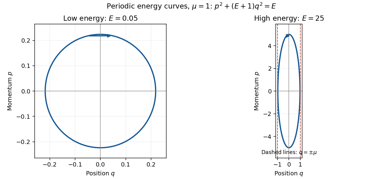

Past exam of the mathematics course of the University of Cambridge 2005 ii Paper 3 15C i Solution Created 2026-09-24 Updated 2026-10-14
The action variable for a regular periodic one-degree-of-freedom Hamiltonian orbit is , with orientation along the motion. Along its energy curve, implicit differentiation gives . Differentiating the loop integral branchwise givesAt simple turning points the two momentum branches join and their endpoint contributions cancel, so the integrable turning-point singularities do not spoil this differentiation. The formula concerns regular periodic levels, not a separatrix of infinite period.
Past exam of the mathematics course of the University of Cambridge 2005 ii Paper 3 14A ii Solution Created 2026-09-24 Updated 2026-10-14
For positive integers , the finite open segment from part (i) works because . For , take a finite closed contour enclosing both branch points , with the integrand analytic in the exterior of the joining cut. Near infinity choose . Since is integral, a circuit around both branch points returns to the initial branch, and the endpoint boundary term cancels. Thus this is an admissible finite contour, including .
For , at that exterior branch is . Deforming the contour to a large circle makes its integral tend to zero; equivalently its Laurent series has no coefficient. Hence . An individual loop around one branch point would not generally return to the same branch when is odd, which is why both are enclosed.
Past exam of the mathematics course of the University of Cambridge 2005 ii Paper 3 14A i Solution Created 2026-09-24 Updated 2026-10-14
Past exam of the mathematics course of the University of Cambridge 2005 ii Paper 3 13E f Solution Created 2026-09-24 Updated 2026-10-14
With response rates and elasticity effectively fixed, changing changes and hence intrinsic noise but not the environmental term. Observation (i) therefore indicates extrinsic noise dominates, making the mean-dependent intrinsic contribution negligible. For a general feedback law whose elasticity changes substantially with the mean, compensation between terms is another possibility; independence from alone would then not logically identify the dominant term.
Observation (ii) measures the local relaxation rate , which is larger under negative feedback. Observation (iii) is not explained by faster adjustment alone. At fixed susceptibility, increasing the response rate increases , reducing time averaging and increasing transmitted environmental noise. Feedback lowers variance primarily by reducing susceptibility and the intrinsic term. Thus rapid adjustment and low noise share a feedback mechanism but are not a direct causal equivalence.
Past exam of the mathematics course of the University of Cambridge 2005 ii Paper 3 13E e Solution Created 2026-09-24 Updated 2026-10-14
For the constitutive system, every propensity is affine in the copy numbers. The exact first- and second-moment equations therefore close: expectations of drift are determined by the means, and covariance drift by the covariance. The stationary fluctuation-dissipation calculation is consequently exact, even though the full joint stationary distribution need not be Gaussian.
For feedback, expectations such as involve nonlinear moments and correlations. Replacing them by a linear expansion about the mean is a linear noise approximation, so the covariance formula is approximate. It works well around a stable single equilibrium when relative fluctuations are small and the rates vary smoothly over their typical range, generally at sufficiently large molecule numbers. Low counts, strong nonlinearities, multiple attractors and proximity to instability can invalidate it.
Past exam of the mathematics course of the University of Cambridge 2005 ii Paper 3 13E d Solution Created 2026-09-24 Updated 2026-10-14
Factor the extrinsic term asThe first factor is environmental relative variance. The second is static susceptibility squared: differentiating the equilibrium relation gives . The last is the time-averaging factor with effective protein response time . Feedback makes response faster, which by itself weakens averaging, but simultaneously reduces the static gain. These are distinct effects and both must be retained.
Past exam of the mathematics course of the University of Cambridge 2005 ii Paper 3 13E c Solution Created 2026-09-24 Updated 2026-10-14
At the deterministic feedback equilibrium use . The indicated elasticity isThe normalized drift becomes ; equal mean birth and death rates still give . Solving the same covariance equation yields the feedback attenuation of gene-expression noise:For , , soThe inverse-feedback expression is interpreted near a positive equilibrium; a microscopic birth rate singular at zero needs a separate regularization there.
Past exam of the mathematics course of the University of Cambridge 2005 ii Paper 3 13E b Solution Created 2026-09-24 Updated 2026-10-14
If RNA concentration does not fluctuate, protein synthesis is an immigration-death process, so its intrinsic normalized variance is . If protein birth/death noise is suppressed and protein responds deterministically to the fluctuating RNA input, the remaining normalized variance isWriting , its factor is . Slow environmental changes are followed almost fully; rapid environmental fluctuations are averaged over the longer protein response time. Thus extrinsic noise is the magnitude of relative RNA fluctuations multiplied by a dynamical averaging factor.
Past exam of the mathematics course of the University of Cambridge 2005 ii Paper 3 13E a Solution Created 2026-09-24 Updated 2026-10-14
Let . The mean equations give and . For relative deviations, the drift Jacobian and normalized reaction-noise covariance areThe normalized stationary fluctuation-dissipation relation for a reaction network is with this negative-drift convention. Its entries successively giveThe birth and death channels act on one species at a time, so the diffusion matrix is diagonal even though the stationary covariance is not.
Past exam of the mathematics course of the University of Cambridge 2005 ii Paper 3 10D c Solution Created 2026-09-24 Updated 2026-10-14
Past exam of the mathematics course of the University of Cambridge 2005 ii Paper 3 10D b Solution Created 2026-09-24 Updated 2026-10-14
For an expanding decelerating power law with , the particle horizon is , and the comoving Hubble radius is . It increases with time, so regions that are mutually visible today can have been out of causal contact at early times. The nearly uniform early thermal conditions inferred across such regions give the horizon problem.
During cosmic inflation, accelerated expansion makes the comoving Hubble radius decrease. A patch initially within one causal communication scale can expand into the region now observed, after which its separated parts are temporarily outside the Hubble radius and later re-enter during deceleration. Sufficient duration before the hot radiation era permits a common causal origin; accelerated expansion is not itself a claim that signals propagate faster than light locally.
Past exam of the mathematics course of the University of Cambridge 2005 ii Paper 3 10D a Solution Created 2026-09-24 Updated 2026-10-14
For a homogeneous isotropic metric, radial light propagation covers comoving distance . The physical particle horizon is , when this is finite. A future event horizon exists when is finite. The Hubble radius is the instantaneous scale , with ; it is not generally the same as either causal horizon.
For an Einstein-de Sitter universe, , so , while from a beginning at zero. The future integral diverges, so there is no event horizon. For an eternal-past de Sitter spacetime, is constant and the particle-horizon integral from diverges. Its event horizon and Hubble radius both equal . Thus a Hubble radius is not automatically a particle horizon, even in these simple isotropic models.
There are unlisted articles, also show them or only show them.