
Past exam of the mathematics course of the University of Cambridge 2015 ii Paper 3 4J Solution Created 2026-09-24 Updated 2026-10-06
The command fits the simple linear regressionusing ordinary least squares. The fitted conditional mean is a straight line in time. The regression residuals are mainly positive at the beginning and end and negative in the middle, so the mean function needs curvature.
A direct improvement is polynomial regression of degree two:The nested-model F-test tests against a nonzero quadratic coefficient. If measurements were used, its statistic isA small reported -value supports the quadratic term. The new regression residuals should then be checked for remaining systematic structure, changing variance and temporal dependence, because the F-test assumes independent errors of common variance. Radioactive decay also motivates an exponential mean, but the displayed curvature already justifies this simple nested comparison.
fit2 <- lm(Counts ~ Time + I(Time^2), data = geiger)
anova(fit1, fit2) Past exam of the mathematics course of the University of Cambridge 2015 ii Paper 3 3G Solution Created 2026-09-24 Updated 2026-10-06
Order the prescribed lengths as . Construct a prefix code on the binary tree. At depth , previously assigned codewords exclude of the vertices. The Kraft inequality impliesso an available vertex can be assigned to the next symbol. None of the assigned words is a prefix of another. Reading each word up to the next assigned vertex gives unique decoding, so this constructs the required uniquely decodable code.
For completeness the same length inequality is necessary even for a uniquely decodable code which is not a prefix code. Write and . For successive symbols, distinct symbol strings have distinct concatenated codewords. At total length there are at most such strings. ThereforeTaking th roots and letting gives . This is the McMillan inequality.
Set . The relative entropy inequality givesHere Shannon entropy uses base , with . The relative entropy is nonnegative, with equality precisely when the two probability distributions coincide; this follows from . Consequently equality holds exactly whenIn particular all alphabet symbols must have positive probability for equality with finite prescribed lengths.
Past exam of the mathematics course of the University of Cambridge 2015 ii Paper 3 38E b Created 2026-09-24 Updated 2026-09-24
Past exam of the mathematics course of the University of Cambridge 2015 ii Paper 3 38E a Created 2026-09-24 Updated 2026-09-24
Past exam of the mathematics course of the University of Cambridge 2015 ii Paper 3 37B Solution Created 2026-09-24 Updated 2026-10-14
For the local phase , define and . The dispersion relation is the Hamilton-Jacobi equation . Differentiate it in space and follow a ray with group velocity ; symmetry of the phase Hessian cancels the terms involving . Thus the ray-tracing equations areHere means differentiation along the moving ray; subscripts on mean partial derivatives holding its other independent arguments fixed.
The depth is stationary and independent of , so and are constant. Choose the incident direction with positive ; the other sign reflects the picture. In the far deep water,Since depends isotropically on the horizontal wavevector, the group-velocity ratio is . Therefore the ray equation isNear shore, , so the shallow-water dispersion relation gives and . Integrating the ray slope yieldsFor , the near-shore phase is . A constant-phase wave crest thus hasIts tangent becomes parallel to the shoreline, while rays approach perpendicular to it. The exponent is between zero and one, giving the curved crests sketched below for .

Near-shore wavecrests bending parallel to the beach and rays approaching normally, for a depth proportional to x
. Details. 
These are the formal geometrical optics asymptotics. For fixed and , arbitrarily close to the shore, so the slowly varying wave approximation eventually fails there; the sketch describes the ray-theory regime before that final inner region.
Past exam of the mathematics course of the University of Cambridge 2015 ii Paper 3 36E iii Created 2026-09-24 Updated 2026-09-24
Past exam of the mathematics course of the University of Cambridge 2015 ii Paper 3 36E ii Created 2026-09-24 Updated 2026-09-24
Past exam of the mathematics course of the University of Cambridge 2015 ii Paper 3 36E i Created 2026-09-24 Updated 2026-09-24
Past exam of the mathematics course of the University of Cambridge 2015 ii Paper 3 35D d Created 2026-09-24 Updated 2026-09-24
Past exam of the mathematics course of the University of Cambridge 2015 ii Paper 3 35D c Created 2026-09-24 Updated 2026-09-24
Past exam of the mathematics course of the University of Cambridge 2015 ii Paper 3 35D b Created 2026-09-24 Updated 2026-09-24
Past exam of the mathematics course of the University of Cambridge 2015 ii Paper 3 35D a Created 2026-09-24 Updated 2026-09-24
Past exam of the mathematics course of the University of Cambridge 2015 ii Paper 3 34A ii Created 2026-09-24 Updated 2026-09-24
Past exam of the mathematics course of the University of Cambridge 2015 ii Paper 3 34A i Created 2026-09-24 Updated 2026-09-24
Past exam of the mathematics course of the University of Cambridge 2015 ii Paper 3 33C b Created 2026-09-24 Updated 2026-09-24
Past exam of the mathematics course of the University of Cambridge 2015 ii Paper 3 33C a Created 2026-09-24 Updated 2026-09-24
Past exam of the mathematics course of the University of Cambridge 2015 ii Paper 3 32A Solution Created 2026-09-24 Updated 2026-10-14
Use the state vector immediately to the right of a delta well. Free propagation to the next well and the derivative jump there areThus the Floquet matrix in this convention isChoosing the state on the other side of each well conjugates the matrix and leaves its eigenvalues unchanged.
The Bloch theorem requires a real quasimomentum with a Floquet eigenvalue . Since , this occurs exactly whenDividing the two inequalities by the positive givesThe upper boundary in is the unique intersection of the increasing line with the strictly decreasing , which runs from infinity to . Call it . The concave function starts with slope and approaches . If , the line has slope at least and stays above it for every , so allowed run from to . If , there is exactly one positive crossing with ; below it the line is inadmissible, and above it the line stays above . Because , . This establishes the negative-energy band of an attractive delta comb: there is exactly one negative-energy band:where , without needing to evaluate the roots.
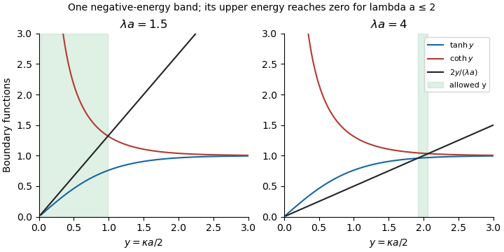
Negative-energy band boundaries from tanh and coth intersections, below and above lambda a equal to two
. Details. 
As with fixed, both positive boundary values of tend to . The band collapses to the isolated delta-well bound state , as tunnelling between widely separated wells disappears.
Past exam of the mathematics course of the University of Cambridge 2015 ii Paper 3 31A Solution Created 2026-09-24 Updated 2026-10-06
With , angular momentum eigenstates have and . Their and eigenvalues are and . Adding spins and gives and, if , . For the Clebsch-Gordan coefficients to be nonzero one requires .
For , write for . The highest state and one application of the angular momentum lowering operator giveThe lowering coefficient of the highest state is , while the two product-state coefficients before division are and . The last line is its normalized orthogonal complement. Its coefficient with maximal is positive, fixing the requested phase convention. All other coefficients for the allowed vanish.
For the decay, the final total intrinsic spin is . Combining it with integer orbital angular momentum to obtain permits only . Parity conservation gives . Thus .
For and initial , the last displayed coupled state shows that the spin-up probability, after ignoring the orthogonal orbital states, is . For , is the maximal coupled angular momentum and its highest state is . Therefore .
Past exam of the mathematics course of the University of Cambridge 2015 ii Paper 3 30E b Created 2026-09-24 Updated 2026-09-24
Past exam of the mathematics course of the University of Cambridge 2015 ii Paper 3 30E a Created 2026-09-24 Updated 2026-09-24
There are unlisted articles, also show them or only show them.