Past exam of the mathematics course of the year 1 of the natural sciences course of the University of Cambridge 2024 Paper 2 16 a Solution by  Codex 0 2026-10-18
 Past exam of the mathematics course of the year 1 of the natural sciences course of the University of Cambridge 2024 Paper 2 15 b Solution by Codex 0 2026-10-18
Codex 0 2026-10-18The associated homogeneous linear differential equation has characteristic roots , so its complementary function is . For a particular integral, the method of undetermined coefficients suggests . Substitution and comparison of coefficients givesso . The general solution is thereforeThe first boundary condition gives . At , the polynomial part already equals the assigned boundary value and the cosine vanishes, so . ThusThis is the unique solution satisfying the two boundary conditions; here the phrase “particular solution” means that selected member of the full family, rather than only the polynomial particular integral.
Past exam of the mathematics course of the year 1 of the natural sciences course of the University of Cambridge 2024 Paper 2 14 c Solution by Codex 0 2026-10-18
Codex 0 2026-10-18The random variable is the sum . The linearity of expectation givesMultiplication by reverses the mean but preserves the variance. Under the independence assumption used in part (b), the variance of a sum givesThus both predictions agree with the direct integrals. For the actual elapsed time, adding twenty-five changes the mean to twenty-five minutes and leaves the variance at minute squared.
Past exam of the mathematics course of the year 1 of the natural sciences course of the University of Cambridge 2024 Paper 2 13 a Solution by Codex 0 2026-10-18
Codex 0 2026-10-18For , the product rule for the curl givesSince , this is not identically zero on . A gradient field has zero curl, so no scalar potential exists for on the whole space.
For the radial vector field , observe thatThus all vector-field potentials areThese are smooth everywhere, including the origin. Any two differ by a constant because their gradient difference vanishes on the connected whole space.
Past exam of the mathematics course of the year 1 of the natural sciences course of the University of Cambridge 2024 Paper 2 12 f Solution by Codex 0 2026-10-18
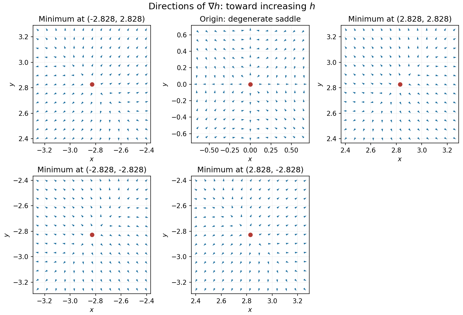
Codex 0 2026-10-18Near a nonzero stationary point , Taylor expansion of the gradient gives . Since the Hessian matrix is positive definite, for sufficiently small nonzero . Thus the gradient arrows point away from each of the four local minima, with different strengths in the two eigenvector directions.
At the origin, on the -axis the gradient is and on the -axis it is , so arrows point outward. On the gradient is , and on it is , so arrows point toward the origin for small . Away from the axes the leading terms are , pointing inward in both coordinate signs. The narrow outward sectors close to the axes are visible in the exact vector field.
Past exam of the mathematics course of the year 1 of the natural sciences course of the University of Cambridge 2024 Paper 2 12 e Solution by Codex 0 2026-10-18
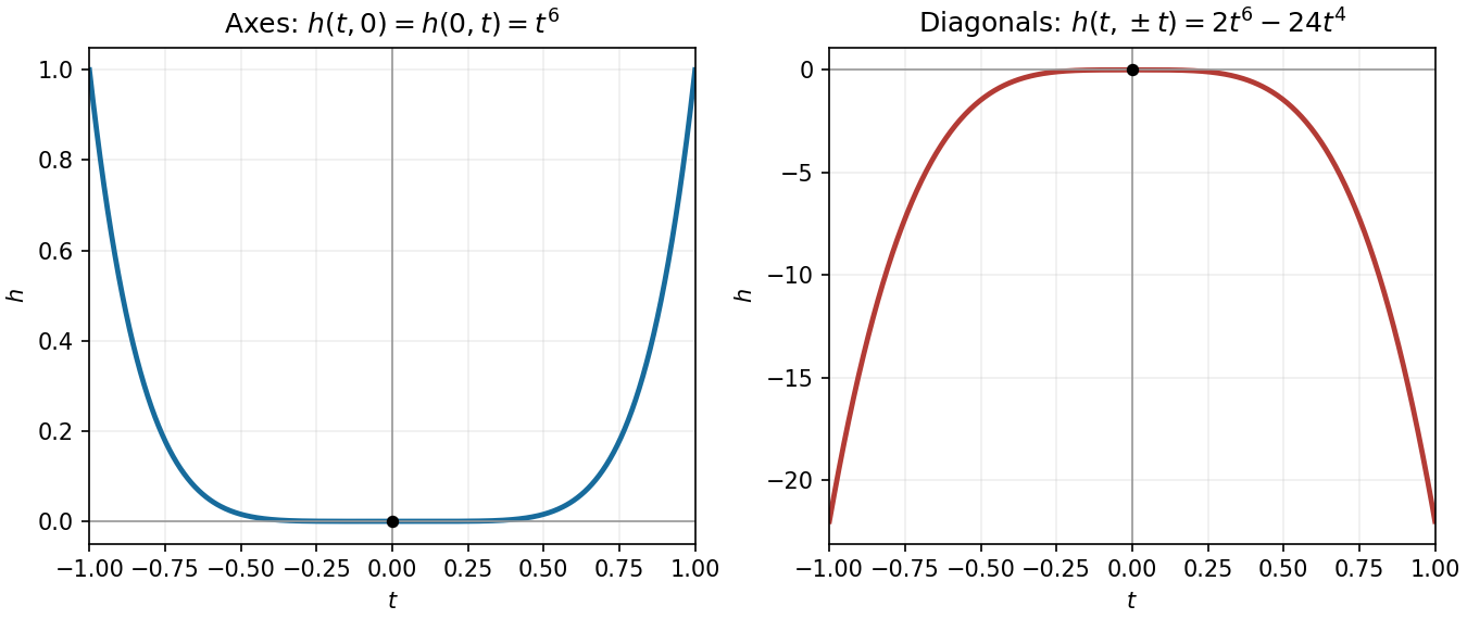
Codex 0 2026-10-18Along either coordinate axis, the restriction is , which is positive for . Along either diagonal it iswhich is negative for sufficiently small nonzero . Therefore every neighbourhood of the origin contains both positive and negative values, whereas . ConsequentlyThe Hessian matrix vanishes there, so the ordinary second-derivative test is inconclusive; the restrictions settle the question.


There are unlisted articles, also show them or only show them.