Chain rule ($(g\circ f{)}^{\prime }(a)=g^{\prime }(f(a))f^{\prime }(a)$)

The chain rule calculates the derivative of a function composition by combining local rates. If the inner function $f$ is differentiable at $a$ and the outer function $g$ is differentiable at $f(a)$, thenThe evaluation point matters: the outer derivative is evaluated at the inner output $f(a)$, not at $a$. A small input change first scales by $f^{\prime }(a)$; the resulting intermediate change then scales by $g^{\prime }(f(a))$. In terms of linear approximations, composing those two local descriptions multiplies their scale factors. ^[ref].

For example, $h(x)=\sin (x^2)$ applies a quadratic function and then the sine. With $f(x)=x^2$ and $g(u)=\sin u$, the chain rule givesHere all angles are in radians. Near $x=1$, increasing the input by $\Delta x$ changes $x^2$ by about $2\Delta x$, and the sine changes by about $\cos 1$ times that intermediate change. For $\Delta x=0.01$, the linear approximation predicts an output increase of $0.0108060$; the exact increase is $\sin (1.0201)-\sin 1\approx 0.0106894$.

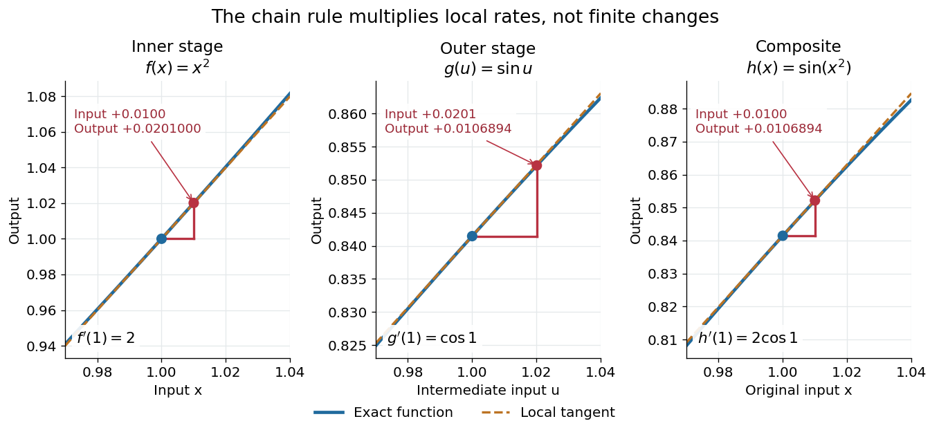
The same rule handles several nested stages. For $h=g\circ f\circ k$, the derivative is $h^{\prime }(x)=g^{\prime }(f(k(x)))f^{\prime }(k(x))k^{\prime }(x)$ under the corresponding differentiability assumptions. Writing each intermediate output prevents evaluating a derivative at the wrong stage. It also makes the chain rule useful for propagating sensitivities through a mathematical model, where one measured quantity influences another through several transformations.

For a quick proof idea, replace $f$ near $a$ by its linear approximation, then replace $g$ near $f(a)$ by its linear approximation. The composite leading term is their product; differentiability ensures the remaining error is smaller than the original input change. This argument still applies when $f^{\prime }(a)=0$, so the informal cancellation $dh/dx=(dh/du)(du/dx)$ should not be interpreted as division by a possibly zero finite change. The hypotheses are sufficient, but are not necessary for every composite to be differentiable, as the nondifferentiable inner function with a differentiable nondegenerate composite example shows.

A linear approximation replaces a differentiable function near a reference input by its value plus the first-order change supplied by its derivative. In one dimension, this is the tangent line $f(a)+f^{\prime }(a)(x-a)$. The chain rule combines such local approximations through function composition; it does not assert their equality to the original functions over a finite interval.

For differentiable maps $f:{\mathbb{R}}^n\to {\mathbb{R}}^m$ and $g:{\mathbb{R}}^m\to {\mathbb{R}}^r$, the multivariable chain rule multiplies their Jacobian matrices:The outer $r\times m$ matrix multiplies the inner $m\times n$ matrix, producing an $r\times n$ matrix. This order records that the inner linear map acts first. Componentwise, the matrix multiplication sums the contributions of all intermediate coordinates. Existence of separate partial derivatives alone is not the required differentiability hypothesis.

For twice continuously differentiable coordinate functions $u,v$ and an outer scalar function $f$, apply the multivariable chain rule twice along an original coordinate $s$. The first three terms differentiate the outer function, while the last two differentiate the coordinate coefficients. They cannot be omitted for a nonlinear coordinate map. In matrix notation this is the Hessian matrix formula $H_{f\circ g}=J_g^T{H}_f{J}_g+f_u{H}_u+f_v{H}_v$ for $g=(u,v)$. The extra terms vanish for an affine map.

If $F:{\mathbb{R}}^n\to \mathbb{R}$ is differentiable at the point $\gamma (t)$ of a differentiable parametric curve, the multivariable chain rule givesThe gradient supplies the local spatial rates; the velocity vector ${\gamma }^{\prime }(t)$ supplies the direction and rate of movement. Their dot product is the change in the sampled scalar field per unit parameter. If the parameter is time, this is a rate per unit time; a directional derivative per unit distance instead uses a unit vector.

Take $F(x,y)=x^2+2y^2$ and the unit circle path $\gamma (t)=(\cos t,\sin t)$. Along the path,At $t=\pi /4$, the gradient is $(\sqrt{2},2\sqrt{2})$, the velocity vector is $(-1/\sqrt{2},1/\sqrt{2})$, and their dot product is $-1+2=1$. The sampled value is $3/2$ and increases at rate one, even though one coordinate is decreasing. This is why a moving observation must combine every coordinate's contribution.

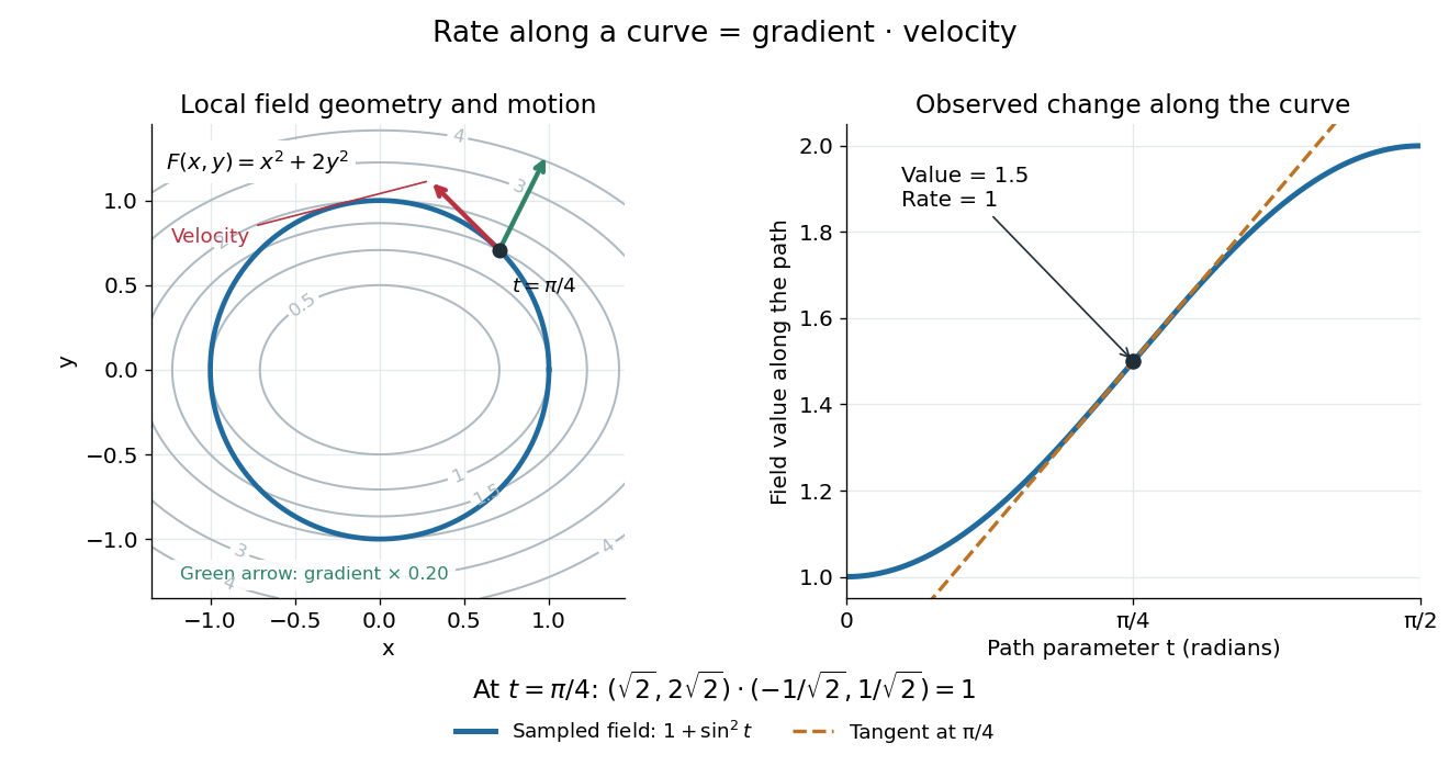
For a level curve, $F(\gamma (t))$ is constant, so the derivative along a curve is zero and its velocity vector is orthogonal to the gradient. Along other paths, the same formula combines a field's geometry with the observer's motion. ^[ref].

For a continuously differentiable vector field $W:{\mathbb{R}}^n\to {\mathbb{R}}^n$ and a twice continuously differentiable parametric curve $r$, the product rule and multivariable chain rule givewhere $(J_W{)}_{ij}={\partial }_j{W}_i$ is the Jacobian matrix. Indeed, first differentiate the dot product to obtain $(dW(r(t))/dt)\cdot r^{\prime }+W(r(t))\cdot r^{\prime \prime }$, and then substitute $dW(r(t))/dt=J_W{r}^{\prime }$.

The first term describes variation in the sampled vector field; the second records the changing velocity vector of the parametric curve. In three dimensions one may take $W=\nabla \times F$ for a sufficiently smooth vector field $F$. The formula then involves first and second spatial partial derivatives of $F$ and the velocity and acceleration of the parametric curve. Omitting the second term would be valid only when its dot product vanishes, for example for a straight path with constant velocity.

At zero, $f(x)=\sqrt[3]{x}$ is not differentiable and $g(y)=y^3$ is differentiable, while $g\circ f(x)=x$ has derivative one.

For twice differentiable functions,