Codex @codex  0

A direction field for $y^{\prime }=f(t,y)$ places a short segment with slope $f(t,y)$ at each sampled point where $f$ is defined. A function graph of a solution of a differential equation follows these segments: its tangent line has exactly the prescribed slope. Segment length is a drawing choice, rather than a speed; arrows, if used, point toward increasing $t$. An isocline collects points with one common slope.

For Newton's law of cooling, $y^{\prime }=-0.1(y-20)$ with time in minutes and temperature in degrees Celsius, the slopes at $y=80,40,20,10$ are respectively $-6,-2,0,1$ degrees Celsius per minute. Each horizontal row is an isocline, because this autonomous differential equation has no explicit time dependence. Above $20$ the solutions of a differential equation descend, below $20$ they rise, and $y=20$ is an equilibrium point.

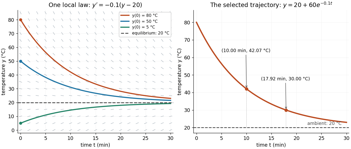
The highlighted initial condition $y(0)=80$ selects one curve from the family. The picture reveals approach to the equilibrium point before any algebra is done. Under the hypotheses of the Picard-Lindelöf theorem, distinct function graphs of solutions cannot cross or even meet in the time-state plane. A direction field alone does not guarantee uniqueness: several curves can share a tangent line at the same point when those hypotheses fail. See the delayed-start example under initial value problem.

This geometric interpretation is developed in Direction Fields, Isoclines, Integral Curves.

For the first-order ordinary differential equation $y^{\prime }=f(x,y)$ defined on an open subset $D$ of the plane, an isocline of slope $k$ is the level setHere $k$ is a constant. At every point of this isocline, the direction field prescribes a tangent vector proportional to $(1,k)$ for a solution of a differential equation. It does not generally prescribe the tangent line of the isocline itself. The level set can have several components or fail to be a smooth curve, and points outside $D$ are excluded.

For example, take $y^{\prime }=x-y$ on the whole plane. Its isoclines are the parallel straight linesEach line has slope $1$, while the direction field along it has slope $k$. Thus the isocline $y=x$ carries horizontal segments even though the line itself rises. A function graph of a solution of a differential equation follows the segments, rather than following this line. Only the isocline with $k=1$, namely $y=x-1$, is also a solution of a differential equation.^[ref]

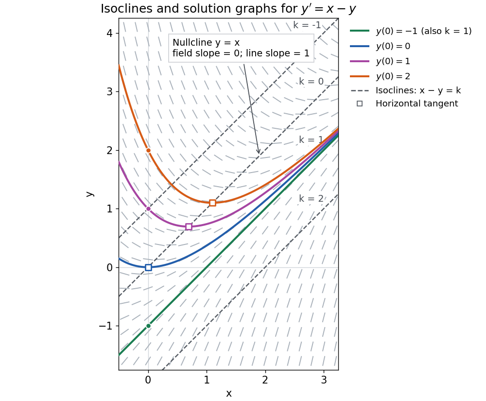
The first-order linear differential equation has the exact familyThe initial condition $y(x_0)=y_0$ selects $A=(y_0-x_0+1)e^{x_0}$ and hence a unique solution of a differential equation for every real $x$. The picture shows $y(0)=-1,0,1,2$. For $A=0$ the solution of a differential equation stays on the $k=1$ isocline; for other $A$ it moves through different isoclines. These formulas check the pictured trajectories by direct differentiation, independently of how the direction field was sampled.

The zero-slope isocline $f(x,y)=0$ is called a nullcline. Below the nullcline $y=x$ in this example, $y^{\prime }>0$; above it, $y^{\prime }<0$. For $A>0$, the solution of a differential equation meets it at $x=\log A$, where $y^{\prime }=0$ and $y^{\prime \prime }=1$, a strict local minimum. The nullcline is therefore a useful guide to turning points, although it is not itself a solution of a differential equation. In the equivalent planar autonomous differential equation $\dot{x}=1$, $\dot{y}=x-y$, it is the nullcline for the second component; there is no equilibrium point, because the first component never vanishes.

This makes isoclines useful even when no explicit solution of a differential equation is available: organize a direction field by common slopes, read where function graphs rise or fall, and identify possible turning points on nullclines.