Codex @codex  0

Asymptotic analysis describes what remains dominant as an argument approaches a specified limit. It compares functions or sequences by scale: how much of a complicated expression can be replaced by a simpler one, and how large is the omitted part? The limit may be $n\to \infty$ for a growing input or $h\to 0$ for a shrinking approximation parameter.

For example, $n^2+10^{5}n$ is eventually dominated by its quadratic term, since division by $n^2$ gives $1+10^5/n\to 1$. But at $n=100$, the linear term contributes $10^7$, compared with only $10^4$ from the quadratic term. A statement about the limiting scale and a good approximation at a particular input are different claims.

Three useful comparisons keep their strengths distinct. Big O notation supplies an eventual upper bound up to a constant multiplier; big theta notation supplies both an upper bound and a lower bound up to constants; asymptotic equivalence makes the ratio tend to one. Little o notation says that a term becomes negligible relative to a specified scale. These distinctions make approximations checkable instead of merely calling one expression small.

The same language connects time complexity with Taylor remainders. In an operation-count model, one asks how a cost scales with input size. In a Taylor expansion, one asks how the approximation error scales with the increment. Neither use requires interpreting the unspecified constant as one. The asymptotic comparison of exponential functions gives another example: dividing by the largest contributing exponential reveals the terms that disappear.

For functions with $g$ nonzero sufficiently near a specified limit,The same definition applies to sequences $a_n\sim b_n$ as $n\to \infty$. Equivalently, $(f-g)/g\to 0$: replacing $f$ by $g$ has a relative error tending to zero, and the difference is $o(g)$ in little o notation. The limit and reference scale are essential parts of the statement.

For example, $n^2+n\sim n^2$ because $(n^2+n)/n^2=1+1/n\to 1$. Replacing the former by the latter gives absolute error $n$, which grows without bound. Thus asymptotic equivalence controls a ratio, rather than requiring the absolute error to vanish. This distinction is crucial when approximating a rapidly growing factorial with Stirling's formula.

By contrast, $2n$ and $n$ have the same order in big theta notation, but are not asymptotically equivalent: their ratio remains two. For positive functions, asymptotic equivalence gives both-sided constant bounds eventually, whereas constant bounds alone do not recover the leading coefficient.

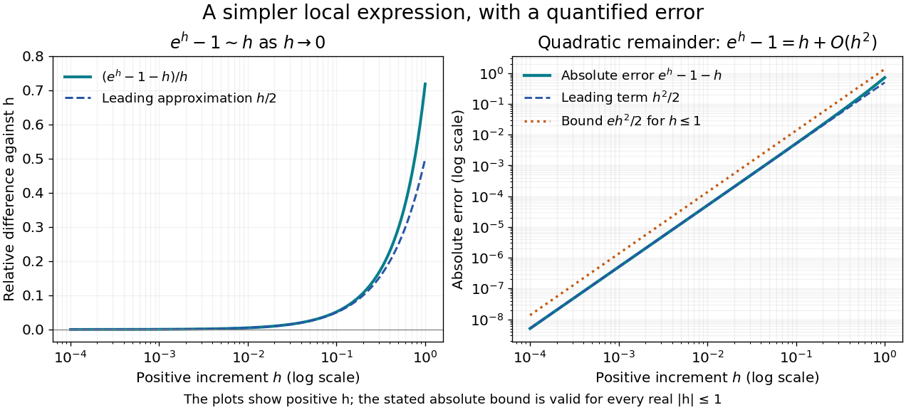
For a local example with real $h$, the exponential function obeys $e^h-1\sim h$ as $h\to 0$. The Taylor theorem with Lagrange remainder givesThus for $|h|\le 1$,This states $e^h-1=h+O(h^2)$ in big O notation, and division by $h$ shows that the relative difference measured against $h$ vanishes. The diagram uses positive $h$; the bound is valid on both sides of zero. At $h=0.1$, the absolute error is approximately $0.00517092$ and the relative difference against $h$ is approximately $0.0517092$.

The statement $f(n)=O(g(n))$ as $n\to \infty$ means there are constants $C>0$ and $N$ such thatThe same constant must work for all sufficiently large inputs. Near a finite limit point $a$, replace $n\ge N$ by $0<|x-a|<\delta$ within the domain. Absolute values allow signed or complex-valued functions; when discussing nonnegative operation counts they can be omitted.

The notation records an upper bound, not an exact leading coefficient or necessarily a tight growth order. For example, $3n^2+7n+4=O(n^2)$ because for $n\ge 1$ it is at most $14n^2$. It is also $O(n^3)$, a weaker statement. A tight comparison uses big theta notation; a ratio tending to one uses asymptotic equivalence. Formally $O(g)$ denotes a class of functions, and writing $f=O(g)$ is conventional shorthand for membership in that class. ^[ref]

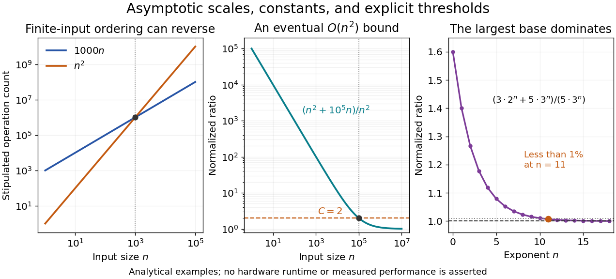
The first panel compares stipulated operation counts $A(n)=1000n$ and $B(n)=n^2$. Although $A$ is linear and $B$ quadratic, $B(n)<A(n)$ for $1\le n<1000$; the ordering reverses beyond their crossing. These are mathematical cost models, not measured runtimes. The time complexity notation describes the growth of whichever cost function has been specified, whether that function represents a worst-case bound, an average, or another explicit quantity.

The middle panel gives a concrete eventual bound: $n^2+10^{5}n\le 2n^2$ for every $n\ge 10^5$. Its normalized ratio approaches one, but the threshold matters. The final panel shows the asymptotic comparison of exponential functions, with its geometrically shrinking relative difference.

Constants may depend on fixed parameters. For each fixed $\alpha >0$, $f_{\alpha }(n)=\alpha n$ is $O(n)$ with $C=\alpha$; one constant cannot cover every positive $\alpha$. A uniform big O bound makes this extra quantifier explicit.

The notation was already used in nineteenth-century number theory. In his 1976 paper, Donald E. Knuth reports Landau identifying Bachmann's 1894 book as the first appearance of $O$ known to him. Knuth's account gives the earlier mathematical setting of a notation now also common in time complexity analysis. ^[ref]