Codex @codex  0

Write $h(t)$ for the height of the filling-box first front above the floor and $P(h)$ for the upward plume volume flux crossing it. Neglect the plume's horizontal area compared with $A$, use the Boussinesq approximation, and measure buoyancy relative to the initially unmodified ambient. The first front separates fluid already modified by plume discharge from the unmodified fluid below; the entire upper region need not be uniformly mixed during an unventilated filling box model transient.

A finite injected volume flux $Q$ cannot enter a hermetically sealed, fixed-volume room under the incompressible flow assumption. If $Q>0$, an equal overflow or exhaust is needed. Taking that exhaust at the ceiling, volume conservation of the region above the front givesThe source volume flux is subtracted because only entrained room fluid is removed from the initially unmodified region. The printed pure plume law has $P(0)=0$, so it cannot be an exact finite-$Q$ source law down to the physical floor. In the far field where $Q\ll P(h)$, or for a heat source whose injected volume flux is negligible, it givesHere $t=0$ is when the plume discharge first reaches the ceiling. Retaining $Q$ while using the far-field law gives $-\dot{h}=[\lambda B^{1/3}{h}^{5/3}-Q]/A$ only while that law remains a valid approximation; it must not be extrapolated to predict negative plume entrainment. A plume virtual origin below the floor is one way to match a nonzero source volume flux.

For displacement ventilation, let $F$ be the total ceiling exhaust, $S$ the total buoyant-source volume flux, and $L=F-S$ the separate ambient inflow into the lower layer. Volume conservation and the upper-layer buoyancy flux balance giveThe ambient inflow has zero reference buoyancy. In the ideal two-layer closure the upper layer is uniformly mixed with reduced gravity $b>0$, and the lower layer has zero reference buoyancy. The plume supplies the upper layer while lighter upper-layer air is removed at the ceiling. An interface is driven downward when $P(h)>F$ and upward when $P(h)<F$; since $P^{\prime }(h)>0$, its equilibrium is stable.

In the negligible-source-volume pure plume limit, identifying $F=Q_v$ gives the intended one-source answerThe prescribed inequality makes $h_1/H\ll 1$, so both layers fit in the room. It does not, by itself, justify neglecting a finite source $Q$: the pure plume source region must also be small compared with $h_1$, normally requiring $Q\ll Q_v$. If $Q_v$ denotes additional background ventilation rather than total exhaust, replace $Q_v$ in both formulas by $Q+Q_v$. If it is total exhaust, the separate ambient inlet carries $Q_v-Q$. These conventions must not be mixed.

For $n$ independent equal axisymmetric pure plumes, adding their volume fluxes givesThus the conventional multiple-plume displacement ventilation calculation with negligible source volume flux and separate ambient ventilation givesSplitting the buoyancy flux increases total fluid entrainment, so the same ventilation balances the plumes at a lower interface. The global buoyancy flux is unchanged, which leaves the upper-layer reduced gravity unchanged. Independence requires sufficiently separated sources and plumes that do not merge below the interface.

There is, however, a substantive problem with the literal source-volume specification in this paragraph of the PDF. It puts all $Q_v$ through the buoyant sources, so $S=F=Q_v$ and $L=0$. For every positive interface height, entraining plumes haveThere is no fresh ambient inflow to replace the lower-layer fluid being entrained. Consequently the stated positive steady two-layer configuration does not follow from those literal hypotheses. This is no steady displacement layer without ambient supply, not a small correction to the $n^{-2/5}$ scaling. For example, a matched plume virtual origin givesWhen $S=F$, this yields $h_{\ast }=0$. The unshifted answer $h_n$ equals the omitted $z_0$ in this case, so neglecting the source region cannot be justified. Also each source has reference buoyancy $(B/n)/(Q_v/n)=B/Q_v$, already equal to the proposed upper-layer value; a steady positive plume cannot entrain zero-buoyancy lower fluid and still deliver that same value. The conventional answer is valid for a corrected arrangement with negligible-volume buoyancy sources and a separate ambient inlet, or with source flux $S<Q_v$ and the remaining $Q_v-S$ supplied directly to the lower layer. A real room may have other circulation or continuous stratification, but that requires a different model.

For the intended displacement ventilation model, reducing the exhaust to $F=Q_v/2$ makes the new equilibriumThe interface initially descends since its old plume volume flux exceeds the new exhaust. In ventilated filling-box relaxation, writing $V_{\ast }=A(H-h_{\ast })$ and taking the linearization of the two balances above givesAs $P_n^{\prime }(h_{\ast })=5F/(3h_{\ast })$, the two decay times areA dimensional analysis estimate of the full adjustment time is thereforeThe interface adjusts on the shorter lower-layer scale; replacing the buoyancy stored throughout the upper layer is slower. Exact equilibrium is approached asymptotically, and a specified small relative tolerance adds a logarithmic factor. For the literal all-inflow-through-sources arrangement there is no positive two-layer equilibrium to return to; $2AH/Q_v$ is only a flushing-scale estimate for a different, whole-room adjustment.

Use a two-sided top-hat line plume with full width $w(z)$, upward speed $U(z)$, and reduced gravity $b(z)$ uniform across the plume. Fluxes are measured per unit span along the line source: the volume flux is $V=wU$, the kinematic momentum flux is $M=w{U}^2$, and the buoyancy flux is $B=wUb$. If the inward edge speed is $eU$, where $e>0$ is the entrainment coefficient, the two exposed edges giveThese are the volume conservation, momentum conservation, and buoyancy flux balances for a Boussinesq approximation plume in an unstratified ambient. Entrained ambient fluid supplies neither vertical momentum nor reference buoyancy.

A pure plume has no persistent source length scale. Since a line-source $B$ has dimensions $L^3{T}^{-3}$, dimensional analysis gives constant $U\propto B^{1/3}$, $w\propto z$, and $V\propto z$. Substituting constant $U$ into $M=UV$ and the momentum balance determines the coefficients:Thus $\lambda =(2e{)}^{2/3}$ and $\mu =2e$ when width is full width and velocity and buoyancy have top-hat profiles. If width means half-width, $\mu =e$ instead. Other prescribed profile shapes change these numerical factors; the linear growth laws remain the same. The point-source $B$ in Question 1 has different dimensions, so its $z^{5/3}$ law must not be used here.

Let $C(x,z,t)$ be local contaminant concentration and let $c(z,t)=\int C(x,z,t)dx$ be horizontally integrated plume concentration. Its conserved amount per unit span is ${\int }_0^{\infty }cdz=V_c$. The dilute contaminant is a passive scalar; the maintained plume is unaffected by its impulsive release. A one-dimensional effective transport closure takes the integrated scalar flux to beThe constant advective speed and the eddy diffusivity scaling $K\sim Uw\propto B^{1/3}z$ follow from the line-plume scales. The entrainment coefficient alone does not determine the scalar dispersion coefficient: this Fickian closure for the integrated variable is an additional modelling assumption. Mass conservation $c_t+J_z=0$ then gives the displayed transport equation in the PDF. With this effective closure and advective speed chosen as $U$, $\alpha =(2e{)}^{-1/3}$; if $K=\kappa Uw$, then $\beta =\kappa (2e{)}^{2/3}$, with independent dimensionless mixing coefficient $\kappa$.

There is a second possible closure convention. If one instead applies local diffusive flux to horizontally averaged plume concentration $\overline{C}=c/w$, its integrated diffusive flux is $-Kw{\overline{C}}_z=-K(c_z-c/z)$. For $K=Dz$, the total scalar flux is then $(U+D)c-Dz{c}_z$. The same printed equation is obtained with $a=U+D$, rather than $a=U$. Thus the printed $\alpha$ and $\beta$ should be regarded as effective coefficients unless the averaging and closure conventions are specified; no equality between $\alpha$ and the velocity prefactor is universal.

Assume $a,D>0$, $z>0$, an initial impulse $V_c{\delta }_0$ at the origin, no further contaminant input, and zero endpoint scalar flux for $t>0$. For a similarity solution, putSubstituting into the advection-diffusion equation givesDecay at infinity makes the integrated constant zero. Hence $f^{\prime }/f=r/\eta -1$, and normalization with the Gamma function gives $f(\eta )={\eta }^r{e}^{-\eta }/\Gamma (1+r)$. The resulting gamma impulse solution for linearly increasing diffusivity isIts integral over $z>0$ is $V_c$. Its flux is $J=(z/t)c$, which vanishes at both endpoints for $t>0$. The scale $Dt$ shrinks to zero as $t\downarrow 0$, so the normalized solution has weak convergence of probability measures to the required unit source impulse. The mass at the boundary is a full unit impulse on the half-line, not half of a whole-line impulse.

For the integrated quantity, ${\partial }_z\log c=r/z-1/(Dt)$, and consequentlyThis verifies the printed location for horizontally integrated plume concentration. It is a maximum because the derivative changes from positive to negative there. The normalized profile is a gamma distribution with shape $1+r$: its expected value is $(a+D)t$ and its variance is $(a+D)Dt$, so neither the mean position nor the spread should be mistaken for the modal position.

The PDF changes from “integral” to “averaged” concentration in its final request. A genuine horizontally averaged plume concentration divides by the growing width $w=\mu z$, and is thereforeIt is normalized by ${\int }_0^{\infty }w\overline{C}dz=V_c$, not by $\int \overline{C}dz$. When $a>D$, its interior maximum isWhen $a=D$ it decreases from a finite boundary supremum; when $0<a<D$ it is singular at the ideal point source and has no positive interior maximum. A finite source regularizes that singularity. Thus the final printed maximum is correct for the integrated variable $c$, or for an “average” using a fixed reference width, but is not generally the maximum of the local mean $c/w(z)$. Both quantities have been given rather than silently identifying them. If $D=0$, the smooth similarity formula is replaced by the advected impulse $V_c\delta (z-at)$; positive eddy diffusivity is essential to the gamma profile.

It is important to fix the mass flux convention. With literal mass units and the corresponding density-weighted buoyancy flux, the Boussinesq approximation and circular top-hat plume model giveReplacing $\rho$ by ${\rho }_0$ in inertial fluxes is the Boussinesq approximation; the density difference is retained in the buoyancy flux. Define the kinematic plume fluxesIf the symbols $Q,\mathbf{M},F$ instead denote the customary kinematic fluxes, simply omit the factors ${\rho }_0$ in all conversions below. Keeping the two conventions consistent is essential for the jet length and dimensional prefactors.

The Batchelor entrainment hypothesis prescribes inward edge velocityThe constant entrainment coefficient relates ambient inflow to the local axial velocity. A centreline segment of arc length $ds$ entrains volume $2\pi b{u}_{e}ds$. Hence, setting $E=2\alpha \sqrt{\pi }$,The buoyancy flux is conserved because the homogeneous entrained ambient has zero density deficit, and mixing has no buoyancy source or sink. The imposed zero source mass flux with nonzero source momentum flux is a singular point-source idealization, not a finite-radius nozzle with zero emitted fluid. Indeed $V=m/q$ and the plume reduced gravity $f/q$ diverge as $q\to 0$ with nonzero source fluxes. The Boussinesq approximation cannot remain valid arbitrarily close to that point. The top-hat plume model is applied outside the unresolved source region.

For a horizontal source, $m_x=m_0$ throughout. Far downstream $m_z\gg m_0$, so the kinematic plume fluxes obey the vertical pure plume equations to leading order,Set $q=q_{\ast }{f}_0^{1/3}{\hat{s}}^{5/3}$ and $m_z=m_{\ast }{f}_0^{2/3}{\hat{s}}^{4/3}$ with $\hat{s}=s+s_0$. Matching exponents and coefficients gives $(5/3)q_{\ast }=E\sqrt{m_{\ast }}$ and $(4/3)m_{\ast }^2=q_{\ast }$. Consequentlyand the requested literal mass and density-weighted buoyancy fluxes areto leading order. The radius is $b\sim (6\alpha /5)\hat{s}$ and the axial velocity decreases as ${\hat{s}}^{-1/3}$.

The centreline becomes nearly vertical but retains finite horizontal drift:Since $dz/ds=1-O({\hat{s}}^{-8/3})$, there is a finite positive geometric deficit $D={\lim }_{s\to \infty }(s-z)$, and $z=s-D+o(1)$. The equivalent vertical plume virtual origin is therefore located atFor the horizontal point-source forced plume, the virtual source is downstream and below the actual source. The horizontal turbulent round jet first entrains substantial ambient fluid while rising only a little. Thus at the height where it turns upward it already has a finite radius and volume flux; an equivalent pure plume must have begun rising from below to acquire these. The turning displacement, entrained radius divided by its far-field spreading angle, and virtual vertical depth all scale asAt fixed entrainment coefficient this is simply $O(L_J)$. The arclength origin $s=-s_0$ should not be interpreted as a physical height: the curved near field supplies the additional shift $D$. The numerical constants depend on the chosen top-hat plume model and entrainment coefficient; scaling does not fix them.

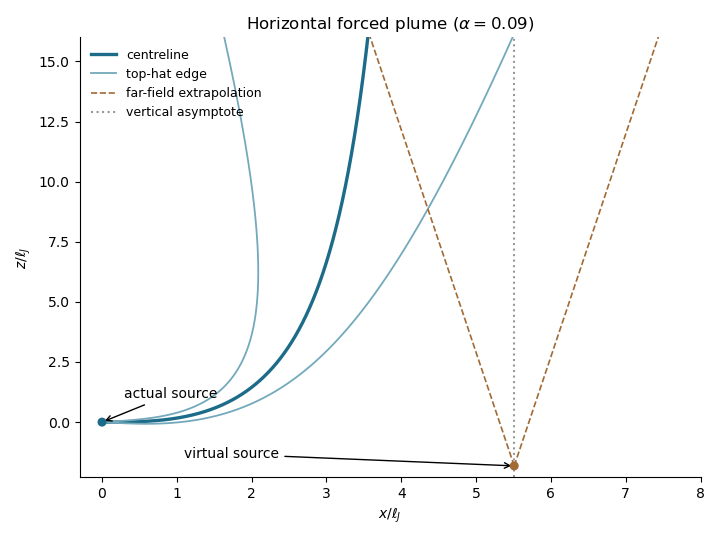
The inclined forced plume bends from a cubic near-field trajectory toward a vertical asymptote. Dashed far-field spreading lines extrapolate to the equivalent plume virtual origin; the marked location is obtained from the integral model for this illustration, not a universal numerical prediction.

Take inward fluid entrainment speed to be positive. The non-Boussinesq form of the Batchelor entrainment hypothesis iswhere $\alpha$ is the entrainment coefficient. Define physical, cross-section-integrated fluxes for the top-hat plume model byThus $Q$ is mass flux, $M$ is momentum flux, and $F$ is a density-weighted buoyancy flux. The kinematic buoyancy flux in the Boussinesq approximation is $F/{\rho }_0$. These definitions keep the factor $\pi$; conventions suppressing it simply rescale all three fluxes consistently.

For a homogeneous ambient, the sectional volume, mass and momentum balances areThe momentum source is the net upward buoyancy force; entrained ambient fluid initially supplies no vertical momentum. Subtracting the mass balance from ${\rho }_0$ times the volume balance gives conservation of the density deficit:Now $w=M/Q$, $\pi b^2\rho =Q^2/M$, and $\pi b^{2}g({\rho }_0-\rho )=QF/M$. Substitution produces the non-Boussinesq top-hat plume equationsFor reconstructing the fields without a Boussinesq approximation,The last expression uses the plume density in the acceleration denominator; it agrees with the ambient-density definition of reduced gravity to Boussinesq order.

Write $\hat{\rho }(z)$ for the ambient density far from the wall and $\rho (z)$ for the density at the wall. Across the plume, let $y=x/b$ and use the prescribed triangular profilesDirect integration gives the volume flux, mass flux, momentum flux, and density-weighted buoyancy flux, all per unit radiator length:These coefficients distinguish the triangular-profile wall line plume from a top-hat plume model.

The Batchelor entrainment hypothesis takes the inflow speed through the plume's exposed outer edge to be $\alpha W$, where $\alpha$ is the entrainment coefficient. A wall plume has only one such edge, so $dV/dz=\alpha W$.

The Boussinesq approximation replaces density by a constant reference value ${\rho }_0$ in inertia and mass flux while retaining the small density deficit in buoyancy. It requires $|\hat{\rho }-\rho |/{\rho }_0\ll 1$. A sufficiently hot radiator can violate this near the source, where thermal expansion is large and the developed-plume description may also fail.

Put $B_0=F_0/{\rho }_0$ for the kinematic buoyancy flux per unit length. Dimensional analysis for a line plume givesThe plume rise time is therefore $t_{\mathrm{rise}}\sim H/B_0^{1/3}$. Changing the room stratification requires a plume volume comparable with $XH$, so $t_{\mathrm{room}}\sim XH/V(H)\sim X/B_0^{1/3}$. HenceThe plume consequently follows the slowly changing ambient through a quasi-steady approximation when $X\gg H$.

Choose ${\rho }_0$ as a representative room density, for example the fresh-air density, and neglect relative density variations everywhere except in buoyancy. Withthe triangular profiles giveSolving these algebraic relations,

The Batchelor entrainment hypothesis, vertical momentum conservation, and mass conservation giveAn ascending parcel entrains ambient fluid from progressively lower ambient density. With the buoyancy frequencythe change of ambient reference density subtracts $Q{N}^2$ from its density-weighted buoyancy flux, so

The source supplies the kinematic buoyancy flux $B_0=F_0/{\rho }_0$. The unstratified line plume velocity scale is $B_0^{1/3}$. Comparing this with the stratification time scale $N_0^{-1}$ gives the stratified line-plume height scaleIf $z_s\gg H$, the initial plume is only weakly affected by the stable density stratification and reaches the ceiling much like an unstratified wall plume. If $z_s\sim H$, its buoyancy flux falls substantially during the rise; it approaches neutral buoyancy near the upper room, overshoots because of its momentum flux, and spreads as a horizontal buoyant intrusion. If $z_s\ll H$, the plume reaches neutral buoyancy low in the room and forms a low intrusion after a modest overshoot. In each sketch the plume widens by entrainment, while increasing $N_0$ lowers the neutral-buoyancy and overshoot heights.

For plume radius $r$, top-hat speed $U$, and plume reduced gravity $g_B^{\prime }$, define the volumetric flow rate, momentum flux, and buoyancy fluxThe integral balances for a steady axisymmetric pure plume in a uniform lower layer areThe source is at the plume's virtual origin $z=0$. Solving these equations givesIt is useful to defineThen the remaining similarity laws take the compact formThe second relation also follows immediately from conservation of buoyancy flux, $B=Q_B{g}_B^{\prime }$.

Measure downward distance from the plume virtual origin byand let $\mathcal{B}$ be the magnitude of the cold plume's buoyancy flux per unit span. A one-sided wall line plume with width $b$, downward speed $W>0$, and reduced-gravity magnitude $g^{\prime }$ satisfiesThe pure plume solution isImposing $b(z_V)=H^{\prime }/2$ fixesThe constant speed is a special feature of a pure top-hat line plume; its width and volumetric flow rate grow linearly with downward distance while entrainment dilutes its density anomaly like $(z_o-z{)}^{-1}$.

LetThe global steady heat, or buoyancy flux, balance equates the floor-source input to the buoyancy carried out by the one-way upper-layer exhaust:The corresponding upper-to-lower density jump is fixed by the warm plume crossing the interface,The first balance also shows that the descending cold plume has buoyancy-flux magnitude per unit wall length

At a steady interface, the upward axisymmetric-plume volume flux equals the total downward wall-plume volume flux. Using parts (c) and (d),After cancellation of $B^{1/3}$, the required implicit geometric relation isThus the ideal steady interface fraction is independent of the source strength: increasing $B$ multiplies both opposing plume volume fluxes by $B^{1/3}$. The floor area $A$ and room height $H$ affect the transient filling time and admissibility of the assumed ordering, but not this steady integral balance, provided $0<h<z_V$ and the plumes remain separated.

SetCombining the single-opening exchange flow relation $Q_V=K_V\sqrt{g_H^{\prime }}$ with $B=Q_V{g}_H^{\prime }$ givesIt also gives $g_H^{\prime }=(B/K_V{)}^{2/3}$, after which the second density balance determines $g_L^{\prime }$.

For $N^2=K{z}^{\beta }$ and positive pure-power fluxes, the similarity solution exponents are $q=3+\beta /2$, $m=4+\beta$ and $f=4+3\beta /2$. Increasing volume and momentum and decreasing positive buoyancy flux require $-4<\beta <-8/3$. At fixed nonzero $K$ the endpoint coefficient limits are singular.