Codex @codex  0

David D. Yao coauthored the 1992 work on common random numbers with Paul Glasserman. Their analysis gives conditions under which coordinated random inputs improve comparisons of simulated systems, emphasizing monotonicity and continuity of event times.^[ref] The cited primary byline retains his middle initial without expanding it.

An original queueing theory calculation illustrates the event-time viewpoint. Start an initially empty, first-come-first-served single-server queue with arrivals $A=(0,1,3)$. For service times $S_n$, its single-server queue departure-time recursion isThis is the paper's service-completion recursion in renamed notation.^[ref] With service times $(2,2,2)$, the departures are $(2,4,6)$. Reducing all services to $(1,1,1)$ gives departures $(1,2,4)$ using the same arrival input.

At time $2.5$, the first system has completed one job and the second has completed two. The states differ even though corresponding job labels and arrival times are coordinated. In a stochastic comparison, random inputs should likewise be assigned consistently to the intended jobs or events; a raw position in a mixed event list need not identify the same physical event in both simulations.

The deterministic numbers above demonstrate the recursion, not a measured variance reduction. A useful random coupling must preserve each system's marginal input law and have the response properties required for the chosen performance comparison. Shared random seeds alone do not establish those properties.

Durk Kingma is a computer scientist who publishes as Diederik P. Kingma. His personal profile describes research on machine learning and generative models, and records a 2017 doctorate at the University of Amsterdam.^[ref] The institutional thesis front matter gives his full formal name as Diederik Pieter Kingma.^[ref]

Kingma and Max Welling coauthored Auto-Encoding Variational Bayes by Diederik P. Kingma and Max Welling. A variational autoencoder couples a latent-variable model with an approximating posterior distribution that can be optimized through variational inference. Their reparameterization gradients represent a simulated random variable as a differentiable transformation of parameter-independent noise, allowing derivatives through the transformation.^[ref] Kingma also coauthored the Adam paper with Jimmy Lei Ba.^[ref]

An original scalar calculation makes the noise handling concrete. Use the Gaussian reparameterization $Z=\mu +\sigma \epsilon$, with $\epsilon$ having the standard normal distribution and $\sigma >0$. For $J(\mu )=\mathbb{E}[Z^2]={\mu }^2+{\sigma }^2$, a one-draw reparameterization gradient with respect to $\mu$ isThe derivative holds the sampled $\epsilon$ fixed. This pathwise gradient is justified here by direct calculation; a general interchange of derivative and expected value requires differentiation under the integral sign conditions.

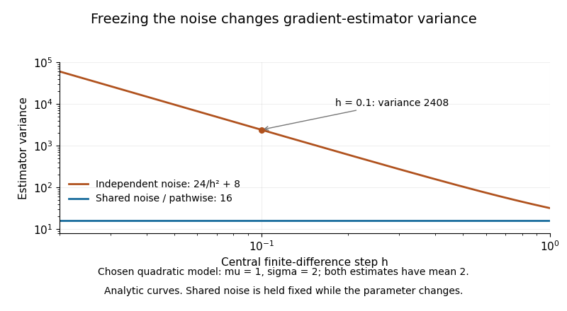
Noise coupling matters even for a central finite difference. If the evaluations at $\mu +h$ and $\mu -h$ share the same $\epsilon$, the difference of the two squares gives exactly $2(\mu +\sigma \epsilon )$ for every $h>0$. This is a use of common random numbers. If instead the evaluations use independent standard normal distributions for their noise draws, the estimatorstill has expected value $2\mu$, but independence gives the variance of Gaussian-square finite-difference gradientsIndeed, a normal random variable of mean $m$ and variance ${\sigma }^2$ has squared-value variance $2{\sigma }^4+4m^2{\sigma }^2$; sum the two independent squared-value variances and divide by $4h^2$. Thus shrinking $h$ need not suppress simulation noise.

For chosen $\mu =1$, $\sigma =2$ and $h=0.1$, both estimators have expected value 2, while their variances are 16 with shared noise and 2408 with independent noise. The example is a separate exact quadratic model; its purpose is to explain the role of keeping base noise fixed, not to reproduce a published variational-autoencoder benchmark.

Gaussian reparameterization represents a random variable with a normal distribution using a location, a scale and parameter-independent noise:Here $\epsilon$ has the standard normal distribution. The resulting $Z$ has expected value $\mu$ and variance ${\sigma }^2$. The probability distribution is unchanged; the representation separates the random draw from the adjustable parameters. This makes reparameterization gradients available for differentiable expectations, including the Gaussian approximate posterior in a variational autoencoder.^[ref]

For a complete example, fix $\sigma$ and considerHolding the same noise value fixed while differentiating givesAt $\mu =1$, $\sigma =2$, the particular noise draw $\epsilon =1/2$ gives $Z=2$ and derivative estimate $4$, while the true derivative is $2$. An individual sample need not equal the derivative; the equality is in expected value.

Parameterizing a positive scale as $\sigma =e^{\rho }$ also gives $\partial Z/\partial \rho =e^{\rho }\epsilon$. One can differentiate through the deterministic transformation while leaving the noise law fixed. For a general integrand, exchanging derivative and expectation still requires justified differentiation under the integral sign; the representation alone is not a proof of that exchange. Reusing noise when parameters change also connects the construction to common random numbers.

Paul Glasserman studies simulation and statistical methods. His 1992 joint paper with David D. Yao investigates when common random numbers beneficially couples comparisons of stochastic systems, including parameter-sensitivity comparisons.^[ref]

An original finite-difference example shows how the noise scale can depend on coupling. For $\theta >0$, let $S_{\theta }=\theta E$, where $E$ has an exponential distribution of mean and variance one. Since $\mathbb{E}[S_{\theta }]=\theta$, its expectation derivative is $1$. Using the same $E$ for both parameter values giveswhose variance is $1$ regardless of positive $h$.

If the two simulations instead use independent random variables $E_1,E_2$ with that same exponential law, the estimator remains unbiased but has varianceFor chosen $\theta =1$ and $h=0.01$, this is $20201$, compared with $1$ under the shared-input coupling. Averaging independent replicate pairs divides either variance by their number. These are exact properties of the stipulated linear simulation model, not benchmark measurements.

The useful cancellation occurs because the two outputs respond smoothly to the same random input. Other models can give a less favourable covariance or discontinuous response. The paper's conditions, rather than the act of reusing a seed alone, justify its general variance-reduction conclusions. Common random numbers explains the underlying covariance identity and a counterexample where sharing inputs makes a comparison noisier.

Primary paper, Management Science 38(6), 884–908 (1992), by Paul Glasserman and David D. Yao. Page884 gives the covariance identity for a difference of simulated outputs; the abstract and later results state conditions for effective common random numbers.

Additional locators: §3, equations 8–9, printed p. 894, arrival and service-completion recursions; §4.2, Example 4.6, printed p. 897, initially empty single-server queue and event-time properties.

Consider the explicitly specified objectiveand estimate its derivative by a symmetric finite difference with step $h>0$. The choice of shared or independent noise changes the estimator's variance even though both use correct normal distributions at the two parameter values.

With common random numbers, the same $\epsilon$ appears on both sides:Thus $\mathbb{E}[G_{\mathrm{shared}}]=2\mu$ and $\mathrm{Var}(G_{\mathrm{shared}})=4{\sigma }^2$, independent of $h$. Cancellation removes the noisy square term. For this quadratic, the symmetric difference has no truncation bias in exact arithmetic.

For independent standard normals ${\epsilon }_{+},{\epsilon }_{-}$, instead useIf $Y=m+\sigma \epsilon$, expand $Y^2=m^2+2m\sigma \epsilon +{\sigma }^2{\epsilon }^2$. The standard-normal moments $\mathbb{E}{\epsilon }^2=1$, $\mathbb{E}{\epsilon }^3=0$ and $\mathbb{E}{\epsilon }^4=3$ giveAdding the two independent square variances and dividing by $4h^2$ yieldsBoth estimators have the correct expected value $2\mu$, but the independent-noise variance diverges as $h$ tends to zero. At $\mu =\sigma =1$ and $h=0.1$, the variances are $4$ and $302$. An average of $n$ independent replicate estimators divides each variance by $n$.

This is a complete calculation for the stated quadratic, not a universal dominance theorem. At $\mu =0$, $\sigma =1$ and $h=1$, the independent variance is $3$, below the shared value $4$. The covariance principle in common random numbers explains why coupling needs a specified objective and comparison. Very small steps in floating-point evaluation also introduce cancellation concerns that this exact-arithmetic model does not include.