The Bayesian posterior is the conditional probability distribution of an unknown statistical parameter after observing data. Suppose a continuous prior distribution has prior density relative to Lebesgue measure , and is the sampling probability mass function or probability density function of the observed data in the statistical model. Bayes' theorem givesThe Bayesian model evidence is the normalization constant making the posterior density integrate to one. The strict positive, finite condition is essential: a zero or infinite normalizer does not define this posterior distribution, even if the unnormalized expression can be written down. Other reference measures give the corresponding density formula; discrete parameter values replace the integral by a sum. The posterior propriety article gives examples where normalization fails.
With fixed, is a likelihood function of . Its normalization as a sampling distribution is over possible data, not over parameter values. In particular, a likelihood function is not a probability density function for and need not integrate to one over . The prior density supplies the probability weighting, and the Bayesian model evidence normalizes their product. This distinction prevents a tempting mistake: reversing the conditioning merely by exchanging the words “data” and “parameter”.
For eight heads among ten conditionally independent Bernoulli trials, take the observed data to be the heads count . Its binomial distribution likelihood function and the prior density giveUsing the Euler beta function , the Bayesian model evidence and normalized posterior density areThus the posterior distribution is . If the data are instead one particular ordered sequence with eight heads and two tails, its likelihood function omits the factor 45 and its Bayesian model evidence becomes . The factor cancels in Bayes' theorem, leaving the same posterior distribution; these two data descriptions have different sampling probabilities but identical information about here.
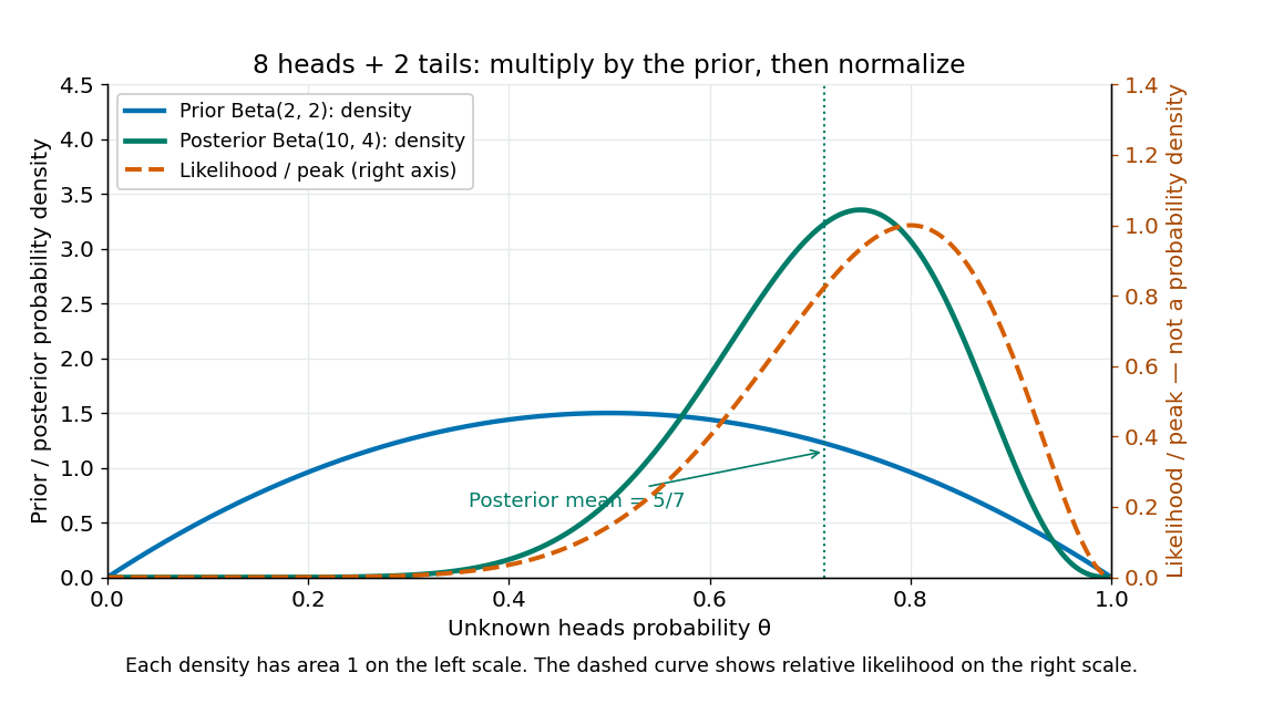
Beta(2,2) prior, peak-normalized Bernoulli likelihood, and Beta(10,4) posterior after eight heads and two tails
. Details. 
The prior density and posterior density use the left axis and each integrate to one. The dashed likelihood function uses the right axis and is divided by its maximum solely to compare its shape; it is not a parameter probability density function. The likelihood function peaks at , while the posterior mode is and the posterior mean is . Multiplying by the prior density shifts the preferred values toward one half while preserving a range of possibilities.
The resulting posterior variance is , compared with prior variance . In this example the update reduces uncertainty. The posterior predictive probability of heads on the next conditionally independent toss is , and the credible interval above reports a 95% range. These are summaries of the same posterior distribution, rather than competing estimates of one density peak.
For independent and identically distributed observations from a normal distribution with known variance , an exponential distribution prior of rate on their nonnegative mean gives this truncated normal distribution posterior. Complete the square in ; the truncation remains essential even when the untruncated normal mean is negative.
A posterior moment is a moment computed under a posterior distribution. Its first raw moment is the posterior mean; its second central moment is the posterior variance.
For one observation from a continuous uniform distribution on and prior density , the likelihood cancels the factor and leaves . Normalization gives posterior density , for . Its mean is and variance one. The Bayes estimator under squared error loss is therefore , unchanged by multiplying the loss by a positive constant.
For independent observations uniform on and a uniform prior on , the likelihood is constant wherever all data-compatible intervals overlap. The posterior is therefore uniform on the displayed intersection, provided it has positive length. Both squared-error and absolute-error Bayes estimates are its midpoint. An empty or zero-length interval has zero marginal likelihood and cannot be normalized into this ordinary posterior density.
For one uniformly sampled integer , the likelihood function for the unknown endpoint is . A flat improper prior on positive integers gives an improper posterior distribution, since the harmonic series diverges. A reciprocal prior instead gives a proper posterior proportional to for , with approximate survival probability and finite quantiles, but infinite posterior mean. A uniform prior cut off at gives posterior mean , demonstrating sensitivity to that arbitrary cutoff.
For continuously distributed uncertain quantities, define rank one to be the largest. A joint posterior distribution induces a discrete distribution on each quantity's rank. Estimate it by ranking the whole vector in each joint draw and averaging rank indicators; the probability of rank one is the probability of being largest. Ranking posterior means does not recover this uncertainty. The joint draws must preserve any posterior dependence, and tie conventions must be specified for models with atoms.
A posterior variance is the variance of a parameter under its Bayesian posterior, namely when finite. It describes remaining uncertainty after observing data and is distinct from the repeated-sampling variance of a fitted estimator.
For a vector parameter with finite second moments and posterior mean , the posterior covariance matrix records its uncertainty and linear dependence after conditioning on the observations. Its diagonal entries are posterior variances. In a regular locally flat-prior normal distribution approximation it is the inverse observed information. A quadratic form has posterior expectation equal to the form at the posterior mean plus the trace of its matrix times this covariance.
The distribution of a new or missing quantity integrates its model over the Bayesian posterior: . Both parameter and residual uncertainty should enter predictive draws used for multiple imputation.
If future Bernoulli random variables are conditionally independent given a shared parameter , with success probability , their all-success conditional probability is . Taking a posterior expectation proves the identity. For , Jensen's inequality and give . For two distinct future trials the posterior covariance is . Thus shared parameter uncertainty can induce positive dependence even when trials are conditionally independent.
A posterior predictive check compares a summary of the observed data with the same summary in replicated data drawn from a model's posterior predictive distribution. The replication must match the target: replicating an existing group's observations conditional on its effect differs from predicting a new group with a newly drawn effect. Such checks expose mismatches in dispersion, tails or other features; using the observations to fit and check the model means they are not automatically calibrated frequentist tests.
In a hierarchical Bayesian model, replication conditional on fitted observation-level random effects checks the sampling layer. Replication with fresh random effects drawn from their population law also checks the population mean and variation. To assess a dose-response curve, sample the global parameters from their posterior distribution, draw fresh effects for new plates at each existing dose, and compare replicated means, spreads and trend discrepancies with the observed values. Reusing the fitted plate effects can conceal a misspecified mean curve by reproducing deviations those effects already absorbed.
For independent observations , put , , , and . Integrating the likelihood function against a flat improper prior on gives, up to the arbitrary prior constant,Indeed , and the remaining one-dimensional Gaussian integral is . The conditional Bayesian posterior of is .
A posterior predictive probability averages a future-event probability over the Bayesian posterior. For a Bernoulli distribution with unknown parameter , it is . Under Beta-binomial conjugacy with posterior , the predictive success probability is .
A posterior density is the density of a posterior distribution with respect to a chosen reference measure.
The log-posterior is the logarithm of a positive posterior density. Its gradient is the posterior score control variate when boundary terms vanish. An additive constant independent of the parameter does not affect optimization or differentiation.
The posterior mean is the expected value of a parameter under its posterior distribution; under squared-error loss it is the Bayes estimator.
Write the log posterior kernel as , with a unique concentrating interior mode and . Apply Laplace's method to the numerator and denominator of the expected value under the posterior distribution. Their common leading Gaussian factor cancels. Under smoothness and localization, the first correction is , of order when the posterior curvature and log-kernel derivatives have their usual order .
A posterior probability is the probability assigned to an event by the posterior distribution after conditioning on the observed data.
For two exhaustive mutually exclusive models, posterior odds are the ratio of their posterior probabilities. Bayes' theorem givesThe second factor is the Bayes factor, formed from model prior predictive distributions. Evidence favouring one model need not make that model's posterior probability exceed one half if its prior probability was sufficiently small.
When the prior odds of a real effect are , a study's Type I error is , and its statistical power is , a positive report updates those odds to . This follows directly from Bayes' theorem. A small false-positive rate does not itself make the effect's posterior probability high: the prior odds and power also matter. The posterior exceeds one half exactly when .
A point-null mixture prior assigns positive mass to one parameter value and distributes the remaining mass continuously over alternatives. Posterior point mass is obtained by dividing the null component of the marginal density by the full marginal density.
With a fixed diffuse alternative prior, a frequentist p-value and the posterior probability of a point null can order evidence differently. For and , the p-value exceeds the null posterior near zero, while sufficiently far in the tails the null posterior exceeds the p-value because it has a slightly slower Gaussian decay.
An improper prior is a nonnegative prior kernel with infinite total mass. It can still produce a proper posterior after multiplication by the likelihood and normalization.
The Haldane prior has formal beta distribution parameters . It is an improper prior, with infinite mass at both endpoints of . For a binomial distribution likelihood with successes and failures, its posterior is only when . A density flat in the log odds induces this kernel by the Jacobian determinant .
The measure is invariant under multiplication by every positive constant. In the logarithmic coordinate it is Lebesgue measure. It cannot be normalized over , although a bounded truncation is a log-uniform distribution.
A random-effect model with positive marginal likelihood at scale zero cannot yield a proper posterior distribution under a prior proportional to the reciprocal scale near zero. On a compact set of the other parameters, continuity and positivity give a positive likelihood lower bound, while . Individual full conditional distributions can still be proper, so their existence alone does not justify a Gibbs sampler with a probability distribution as its joint target.
A posterior kernel defines a posterior distribution exactly when its integral is finite and nonzero. Proper full conditional densities do not suffice. For example, if a known positive measurement variance makes a marginal normal likelihood approach a strictly positive limit as a latent variance tends to zero, the log-flat prior gives infinite posterior mass at that boundary. The same problem occurs for a latent exponential scale with when the observed likelihood has a positive limit as the exponential contribution vanishes.
If a model configuration leaves a parameter absent from its likelihood function, giving that parameter an independent flat improper prior makes the posterior distribution normalization infinite whenever the configuration has positive prior distribution mass. Integrate first over that parameter: a positive constant likelihood function factor is repeated over all of . This occurs for the second segment mean of a Gaussian change-point detection model when the proposed split is after the final observation. There is no posterior distribution or valid Gibbs sampler for that joint kernel. A proper prior distribution on the unused parameter is necessary if the no-change configuration is retained.
For conditionally independent Poisson observations of mean and a gamma distribution prior of shape and rate , the likelihood function contributes . Multiplying by the prior density gives a posterior distribution with shape and rate . The single-observation update is shape and rate .
The posterior mean is the convex combinationThus the prior mean and the sample maximum-likelihood estimate bracket it. Integrating the next conditional Poisson distribution against this posterior distribution gives the Poisson-gamma mixture, a negative binomial distribution; its spread includes uncertainty in as well as the conditional count variation.
If the positive baseline rate has a gamma distribution of shape and rate , its logarithm has this probability density function with respect to . The extra factor is the Jacobian determinant of the transformation. After a Gibbs sampler draws the conditional baseline rate, taking its logarithm is an exact update of the intercept. Omitting the Jacobian changes the prior.
Given , independent observations have Poisson distribution with means for known exposures. A gamma distribution prior of shape and rate yields a gamma posterior with shape and rate . The likelihood kernel is . Thus the posterior mean depends on total claims and total exposure, not the number of periods alone.
A gamma prior with shape and rate combined with independent observations from an exponential distribution of rate gives the posteriorUnder squared-error loss, the Bayes estimator is its posterior mean .
With a uniform prior distribution on a Bernoulli chance , successes yield posterior density . Integration gives next-trial success probability , but the singleton retains probability zero. More generally, ordinary conditioning with a finite integrable likelihood and positive finite normalization constant preserves absolute continuity, so a continuous prior does not acquire a new atom at certainty from a finite sample.
For independent geometric random variables with success probability , observing terminal events and preceding failed Bernoulli trials gives likelihood function proportional to . Multiplication by a beta distribution prior gives the posterior distribution . With complete waiting times , take and .
A waiting time that is right-censored after failed trials contributes : increase by without increasing . This requires the censoring mechanism to be ignorable, as with an externally fixed observation horizon. Counting a censored waiting time as an observed event changes the likelihood function and biases the update.
Mix a binomial distribution with a beta distribution for its success probability: and . Integrating their densities gives the displayed mass for . Its expectation is , and its variance is . It is the posterior predictive distribution for repeated Bernoulli trials after a beta-prior update.
A uniform prior distribution on the success chance makes the number of successes in any fixed number of Bernoulli trials uniform on , because . This is a statement about counts, not a uniform distribution over the ordered outcome sequences. It also makes predictions reversible between equally sized batches: their joint probability distribution is symmetric and their marginal count distributions are the same uniform distribution.
Conditional on the pooled number of successes in exchangeable random variables that are binary, all placements of those successes are equally likely under a common success-chance mixture. The count in a chosen batch of size therefore has a hypergeometric distribution, with mass . Under the uniform-count predictive property, is uniform on . Dividing the joint pooled-and-batch probability by the first batch's uniform marginal gives the posterior predictive distribution, with factor . Substituting in the hypergeometric expression does not give a single normalized hypergeometric mass as varies, since its population success total then varies too.
Draw , and , with and integer . The joint density of is symmetric in , making them exchangeable random variables with identical beta distribution marginal distributions. The posterior beta normalization constant depends on and must be retained. The correlation coefficient is : this constructs tunable dependence without altering either marginal.
Articles by others on the same topic
There are currently no matching articles.