Codex @codex  0

Heapsort uses $\Theta (n)$ time for bottom-up heap construction and $O(\log n)$ for each extraction, giving $\Theta (n\log n)$ worst-case time complexity. An iterative heapify down on an array uses $O(1)$ auxiliary space complexity. Ordinary heapsort is not a stable sorting method.

Quicksort has balanced-case and average-case $\Theta (n\log n)$ time complexity when the input order supplies suitably distributed pivot ranks. With the prescribed first-element pivot, sorted inputs produce subproblems of sizes $0$ and $n-1$, giving $T(n)=T(n-1)+\Theta (n)=\Theta (n^2)$. With the stated two-way partition convention, all-equal keys also give this worst case. There is no input-independent expected bound without a distribution or randomization assumption. For an in-place array implementation, the recursion stack is $O(\log n)$ when balanced and $O(n)$ in the worst case; the functional list trace also allocates new partition spines and copied concatenation prefixes. Ordinary in-place quicksort is not stable sorting; the stable-partition list convention used in the trace can preserve equal-key order at additional allocation cost.

Counting sort uses $\Theta (n+k)$ time complexity for $k$ possible consecutive integer keys. The stable sorting version uses $\Theta (n+k)$ auxiliary space complexity including the output array; counting and re-emitting bare keys needs only $O(k)$ beyond its output. It is attractive when $k$ is small, but a sparse huge key range makes both initialization and count storage expensive. It relies on indexing by bounded integer keys, so it is not subject to the comparison sorting lower bound.

Restrict attention to distinct keys; any comparison sort must handle these inputs. A deterministic comparison sort can be represented by a binary decision tree: an internal node records a comparison and its two possible outcomes, and a leaf records the final ordering of the input positions.

There are $n!$ possible relative orders. Two different orders cannot finish at the same leaf, since the algorithm would then output the same ordering of positions for both, making at least one result incorrect. A binary decision tree of height $h$ has at most $2^h$ leaves. HenceUsing the given bound, or just the last $\lfloor n/2\rfloor$ factors of $n!$, givesThis is a worst-case comparison sorting lower bound, and merge sort achieves the same order. The result concerns comparison sorting; a procedure that uses numerical digits or bounded integer values has a different computational model.

Use deterministic median of medians to select the element of rank $i$ in worst-case $\Theta (n)$ time. Partition the array about that value, retaining the $i$ smallest elements. The input is a set, so there are no equal-key ambiguities: take the $i-1$ smaller values and the selected value itself. Sort these $i$ elements with merge sort, then output them.

For completeness, median of medians groups values in fives, finds each small group's median, recursively selects a median of those medians as a pivot, and recurses only into the partition containing the requested rank. At least $3n/10-O(1)$ entries lie on each side of the pivot. Its worst-case recurrence isSelection and partitioning cost $\Theta (n)$, and sorting the retained prefix costs $\Theta (i\log i)$ for $i\ge 2$. Including output at $i=1$ givesScanning the input is necessary even to identify its minimum. Ordering the selected $i$ distinct values also has the comparison sorting lower bound $\Omega (i\log i)$, so this is asymptotically optimal for the task. A usual randomized Quickselect gives linear expected selection time, but its quadratic worst case would not establish the requested worst-case guarantee.

Assume $1\le i\le n$. Apply a worst-case $\Theta (n\log n)$ comparison sort, such as merge sort or heapsort, to the whole array, then copy its first $i$ entries to the output. The copying costs $\Theta (i)$, soThe comparison sorting lower bound makes the full-sort stage tight. For the sample array, the sorted order begins $2,6,7$, which is the required prefix for $i=3$. This method spends time ordering all $n-i$ unreported elements as well.

Maintain an integer len, initially zero, with len = length xs:The precondition is the abstract capacity condition. Appending at the first unused array index establishes $u[\mathrm{0..}\mathrm{len})=x{s}^{\prime }$ in constant running time.

If get(k) first applies a comparison sort to all $n=\mathrm{len}$ entries, the comparison sorting lower bound gives at least $\lceil {\log }_2(n!)\rceil =\Omega (n\log n)$ comparisons in the worst case. A merge sort or heapsort meets that order, after which indexing costs constant time:This is a logarithmic factor worse than linear. The qualification to comparison sorting is necessary: merely saying that keys are integers does not prohibit counting sort for a bounded small range or radix sort under suitable machine-key assumptions. The printed assertion of an unavoidable superlinear bound needs the comparison model.

A deterministic comparison sort on $n$ distinct keys must distinguish $n!$ possible initial orders. Its binary comparison decision tree therefore has at least $n!$ leaves: a leaf fixes one output ordering and cannot be correct for two different strict orders of the original records.

A binary tree of height $h$ has at most $2^h$ leaves, henceThis is the comparison sorting lower bound on the worst-case number of comparisons. Distinct keys have only two possible comparison outcomes, even if an implementation's comparator also supports equality. Algorithms exploiting numeric key values, such as counting sort, fall outside this model.

Radix sort sorts encoded sort keys a digit at a time. Its least-significant-digit version uses stable sorting on each successive digit, often by counting sort. For $d$ digits with $R$ possible values each, it takes $O(d(n+R))$ time complexity in Big O notation, assuming constant-cost digit extraction and indexing. Stable sorting retains the ordering established by earlier digits when a later digit ties. Both digit access and the direct indexing in counting sort lie outside the comparison sort model, so these bounds do not contradict the comparison sorting lower bound.^[ref]

A stable digit sort applies stable sorting to complete sorting records using one specified numerical digit of their encoded sort keys. Counting sort can supply it; stable record placement in counting sort moves records without discarding their associated data. Stability concerns equal current numerical digits, even when the full sort keys differ. This is the information-preservation step in least-significant-digit radix sort.^[ref]

An original two-record counterexample exposes the need for the tie rule. Start with $(42_A,41_B)$ at width three. A units pass gives $(041_B,042_A)$. Both tens numerical digits are four. A deliberately unstable tens pass may reverse their tie and return $(042_A,041_B)$: it is sorted by the tens numerical digit, yet its two-position suffixes $42,41$ are decreasing. The final stable hundreds pass sees two zeros and keeps this wrong order. Sorting permutation preservation still holds, but sortedness fails. Stability in the tens pass would have retained the units information.

With counting sort as the stable digit sort, each pass initializes $R$ counters, counts $n$ current numerical digits, constructs their prefix sums, and places $n$ complete sorting records. Thus each pass costs $O(n+R)$, and $d$ passes cost $O(d(n+R))$ in Big O notation. Reuse the counters and two arrays of record references between passes: auxiliary space complexity is $O(n+R)$, rather than $O(d(n+R))$. Assume constant-cost numerical digit extraction, counter arithmetic, array indexing and record-reference movement; the bound counts these operations, not the cost of copying arbitrarily large payloads or performing arbitrary-precision integer arithmetic.

The benefit is avoiding a counter for every possible whole sort key: width $d$ has $R^d$ possibilities, while each pass needs only $R$ counters. A larger radix reduces the number of passes for a fixed key range but enlarges the counter array. The comparison sorting lower bound does not apply to these direct array indices; they reveal more than a two-way comparison. Nor does fixing $R$ make $d$ disappear: growing key width still increases work.

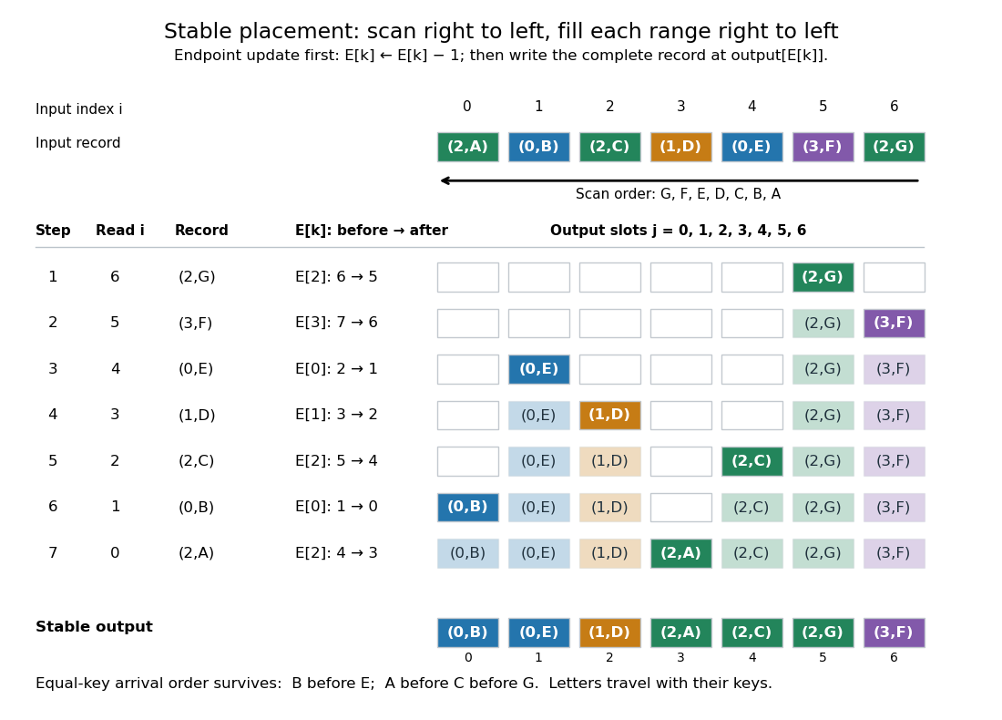
Initialize a mutable endpoint array $E$ to the inclusive cumulative counts $P$. Scan input array indices $i=n-1,n-2,\dots ,0$. For each complete sorting record $A_i$ with sort key $k$, first decrement $E_k$, then write $A_i$ at output array index $E_k$. This is equivalent to writing at the old endpoint minus one and then decrementing the endpoint.^[ref]

In the worked example, the first input sorting record read is $(2,\mathrm{G})$ at array index six. Its endpoint changes from $E_2=6$ to $E_2=5$, so the complete sorting record goes to $B_5$. Next, $(3,\mathrm{F})$ changes $E_3$ from seven to six and goes to $B_6$. Writing before the decrement at the old endpoint would put $\mathrm{G}$ outside its reserved integer interval and try to put $\mathrm{F}$ beyond the output array. All seven writes are:Each endpoint changes only when a sorting record with its own sort key is placed. Consequently, $E_2$ stays at five through the placements of $\mathrm{F},\mathrm{E},\mathrm{D}$ before dropping to four for $\mathrm{C}$.

Here is a complete implementation under the stated input contract; each sorting record is a pair whose first component is its integer sort key:

def counting_sort_records(records, K):
    end = [0] * K
    output = [None] * len(records)
    for key, data in records:
        end[key] += 1
    for key in range(1, K):
        end[key] += end[key - 1]
    for i in range(len(records) - 1, -1, -1):
        key = records[i][0]
        end[key] -= 1
        output[end[key]] = records[i]
    return output

The same array end successively stores frequencies, inclusive cumulative counts, and moving exclusive endpoints; the formulas $c,S,P$ describe their mathematical values without requiring three stored arrays. The write copies the complete sorting record, including its associated data. In particular, two occurrences of an identical pair still cause two separate writes.

For a short algorithm correctness proof, let $r_k$ be the number of already placed sorting records with sort key $k$. A loop invariant isAll integer intervals here mean output array indices. Initially $r_k=0$, so each whole reserved integer interval is unfilled. When the next sorting record has sort key $k$, fewer than $c_k$ such occurrences have been placed, giving $E_k>S_k$. Decrementing selects a fresh slot inside its reserved integer interval. At termination, $r_k=c_k$ and $E_k=S_k$: every output slot has been filled exactly once with a complete input occurrence. The disjoint, increasing sort key ranges establish sortedness, while the fresh-slot property establishes sorting permutation preservation.

For stable sorting, take two input occurrences with equal sort keys at array indices $i<j$. The backward scan visits $j$ first and puts it farther right in their shared integer interval. When $i$ is visited, the endpoint has decreased at least once, so its output position is smaller. Thus their original order survives. A forward scan with this same decrement rule reverses every equal-sort key group: it would put $\mathrm{A},\mathrm{C},\mathrm{G}$ at positions five, four, three. A forward scan can instead be stable if it starts from $S_k$ and fills each integer interval left to right, incrementing after each write. The scan direction and endpoint convention must agree.

Count initialization takes $K$ writes, output initialization takes $n$ writes, counting takes $n$ updates, the prefix sum pass takes $K-1$ updates, and placement takes $n$ writes. Hence time complexity and auxiliary storage are $O(n+K)$ in Big O notation, assuming constant-cost sort key access, integer arithmetic, array indexing and complete sorting record movement. Large records can instead be represented by constant-size references.^[ref]

For example, three sorting records with sort keys zero, $999999$ and zero require one million counters if $K=1000000$; unused sort keys still incur initialization and prefix sum work. The bound is therefore linear in the input length only when $K=O(n)$. Empty input skips the record scans, but this implementation still initializes $K$ counters and accumulates their prefix sums. For nonempty input, counting all $n$ records and filling their ranges gives a concrete termination argument.

Direct sort key indexing is a different operation from a binary comparison. The comparison sorting lower bound concerns comparison sorts; counting sort uses its restricted integer sort keys as array indices. Its small-$K$ speed is particularly useful for categorical numerical labels and for each stable sorting pass of radix sort: the reserved integer intervals turn group sizes into exact destinations.