Codex @codex  0

A complex cell typically responds selectively to an oriented edge or bar over a finite spatial region with less dependence on spatial phase and contrast polarity than a simple cell. It need not have the simple cell's separated linear ON and OFF subregions. Phase tolerance is local, not invariance to arbitrary displacement outside its receptive field.

Fit a stimulus-conditioned linear-nonlinear-Poisson cascade model. Choose a causal stimulus-history window, subtract the stimulus mean, and estimate a temporal filter $k$. A useful initial estimate is the spike-triggered average, $\hat{a}(u)=N^{-1}{\sum }_i[s(t_i-u)-\bar{s}]$. For white Gaussian stimulation and a one-filter response, this estimates the filter direction. With correlated Gaussian stimulation it estimates a direction proportional to $Ck$, where $C$ is the history covariance matrix; use stimulus-correlated spike-triggered averaging to whiten or regularize this correction. An arbitrary stimulus or an even response nonlinearity does not guarantee that this average identifies the correct model.

A general fitting approach is to expand a causal filter in smooth basis functions, compute $a(t)=b+{\int }_0^{U}k(u)s(t-u)du$, and take a nonnegative rate $\lambda (t)=f(a(t))$. With $f(a)=e^a$, fit the coefficients by Poisson spike-train likelihood fitting:The first term rewards rate at observed spikes and the second penalizes overprediction elsewhere. Include a filter-size or smoothness penalty, and choose complexity on held-out data. Another option estimates $f$ by stimulus-projection histograms: divide the density of projection values at spikes by their occupancy density, multiplied by the mean firing rate. Avoid interpreting poorly sampled bins as reliable rates. Temporal train/test splits should avoid leakage through the filter-history window.

Given the fitted rate and the same stimulus, generate an Inhomogeneous Poisson process. For small bins of width $\Delta t$, spike with probability $1-e^{-\lambda (t)\Delta t}$, choosing the bins sufficiently short that multiple events are negligible. More exactly, advance integrated intensity until it increases by an independent unit-exponential random variable, then place the next event. Repeating this generates different synthetic spike trains with the same fitted stimulus-dependent rate, not copies of the original event times.

Compare held-out log-likelihood, stimulus-conditioned firing-rate predictions, count distributions, interspike-interval distributions and autocorrelation. With repeated identical stimulus presentations, compare trial-averaged time courses and trial-to-trial count variance, including the Fano factor. A single recorded train does not by itself supply a reliable repeated-trial average or variance; use held-out temporal data, model-based uncertainty and further recordings instead. Time-rescaled spike-train diagnostics test whether integrated-intensity intervals look independently exponential, rather than comparing raw intervals to an exponential law under a changing rate.

A successful model reproduces specified statistical features on new data; identical spike times are not the goal. The basic Poisson model can miss refractoriness, bursting, adaptation, history dependence or stimulus-unexplained trial variability. If needed, add a spike-history filter to the conditional rate, including an absolute dead time, and fit the resulting history-dependent model. A complex cell may also require multiple filters or quadratic stimulus features: its spike-triggered mean can vanish despite strong tuning. These failures identify model limitations rather than evidence that a random spike generator should match every observed interval.

A complex cell in primary visual cortex typically responds to a suitably oriented bar, edge or grating over a finite receptive-field region, with less dependence on precise spatial phase and contrast polarity than a simple cell. Its response need not reveal separated linear ON and OFF subregions. Many cells have additional motion or binocular selectivity, so phase tolerance alone is not a complete account of every complex cell. Moving the feature beyond its receptive field still reduces the response.

In a pooling model of a complex cell, several simple cells with similar preferred orientation but different positions or phases feed the output. For linear subunit responses $a_m=⟨k_m,I⟩$, a possible model is $r=f({\sum }_m{w}_m[a_m-{\theta }_m{]}_{+})$, with $w_m\ge 0$. Include opposite-polarity filters if both light and dark features are to drive the cell. Rectification stops cancellation between subunits, and pooling spreads position and phase sensitivity across their coverage.

In a quadrature energy model of a complex cell, use two oriented filters of matching frequency but quadrature phase, and setFor a matched grating, choose the pair so $a_e=A\cos \phi$, $a_o=A\sin \phi$; then $E=A^2$, independent of grating phase while retaining orientation and frequency tuning. Finite approximate filter pairs give only approximate invariance for general images. The quadrature construction underlies the primary Adelson–Bergen energy-model work; temporal filters can extend it to motion sensitivity.

The pooling model emphasizes a circuit of rectified subunits and can flexibly cover translated positions. The energy model gives an explicit algebraic phase-invariance mechanism with quadratic contrast dependence before its output nonlinearity. They are not mutually exclusive biological alternatives: suitable subunit pooling can approximate an energy computation. Their spatial tolerance, contrast response and direction selectivity depend on the chosen filters and nonlinearities, and both require comparison with measured receptive fields.

A simple cell is a visual cortical neuron whose receptive field has spatially separable ON and OFF receptive-field subregions. Elongated neighboring subregions give a preferred orientation and a sensitivity to the location and polarity of visual contrast. “Simple” describes the response organization; it does not describe a simpler cell body or a particular shape of neuron.

Hubel and Wiesel's 1962 classification emphasized four observations: distinguishable ON and OFF receptive-field subregions, summation within each region, antagonism between regions, and qualitative prediction of responses to differently shaped stimuli from those regions' arrangement. A slit fitting an elongated center was more effective than a smaller spot; a larger patch could invade opposing flanks and lose effectiveness. An edge separating bright and dark regions could be effective when its boundary matched the boundary between subregions. These were observations about spike trains, rather than an assertion of exact linearity. ^[ref]

The following deliberately coarse signed spatial filter model of a simple cell makes the geometry easy to count. A centered bright bar contributes positively at five sites. Rotating it preserves its area but mixes positive and negative weights; shifting it preserves its orientation but changes which weights it samples. The model is useful because it predicts distinct effects of these three manipulations instead of treating any bright stimulus as equivalent.

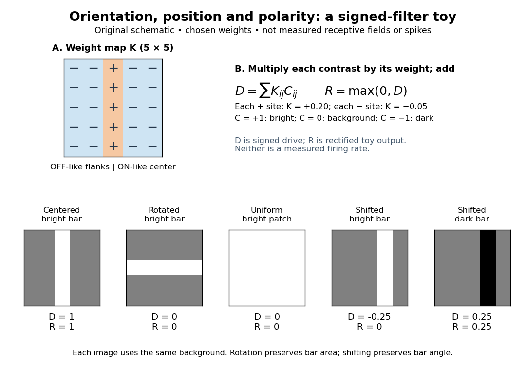
A simple cell is not an ideal linear sensor. Its spike train is nonnegative in event count, and neural adaptation can change responsiveness. The signed spatial filter model of a simple cell supplies a useful approximation to spatial drive and an explicit output rule. Comparing predictions with unseen stimuli is more informative than assuming the rule from the name “simple”. In contrast, the existing complex cell models explore tolerance to phase and local displacement.