Contact-mode timestep stability concerns whether a numerical integrator introduces growing errors when advancing the fast dynamics of an active penalty contact. It depends on the integration rule and the local modal frequencies, not just the size of the modeled overlap. The primary compliant-contact treatment identifies stiff contact springs as a source of numerically stiff differential equations.[ref]
Underactuated Robotics by Russ Tedrake. Multi-Body Dynamics, Compliant Contact Models, stiff-spring and numerical integration discussion
Freeze the active contacts and linearize about a compressed equilibrium. An undamped mode has . For step , put . The Forward Euler method updates displacement and velocity with matrixwhose eigenvalues are . Their magnitudes are whenever . Thus the method has no nonzero stable step for indefinite integration of this undamped oscillator, although smaller steps reduce its error on a fixed finite interval.
The central-difference recurrence instead givesFor its two distinct amplification roots lie on the unit circle. At the repeated root is , and solutions can include , so the strict bound matters. A collection of frozen undamped modes therefore requires for this oscillatory stability condition. In coupled normal-contact penalty modes, comes from the coupled system rather than an arbitrary total-mass estimate.
Stability still allows substantial contact-mode numerical phase error. For central differences the phase per step is , giving numerical angular frequency . At and , is stable but the numerical frequency is about , high. A timing-sensitive contact event can consequently drift even when oscillation amplitudes do not grow.
Implicit schemes illustrate another tradeoff. For the Backward Euler method, the amplification factors are and have magnitude . At , each step reduces the oscillatory amplitude by about , despite the continuous undamped system conserving energy. The trapezoidal rule instead has factorswith phase . The same example gives , low. Unconditional stability for this linear model does not imply correct timing at a large step.
A practical error check therefore compares both amplitude and phase while reducing . For instance, a small target dimensionless step gives much smaller phase error than one, but the acceptable value depends on the observable and time span; it is not a universal accuracy certificate.
The frozen-mode argument has a defined scope. Contact opening changes the active stiffness, nonlinear force laws change tangent stiffness, and damping introduces additional eigenvalue scales. An integrator can satisfy the local oscillator bound while missing an intervening collision or contact release. A proposed test starts with a small compressed-contact perturbation, checks frequencies and energy behavior, then repeats across a known contact-opening event with decreasing steps. Record force histories and event times as well as penetration, so numerical damping or phase drift is not mistaken for a material response.
Contact-mode numerical phase error is the difference between the oscillation phase produced by a time integrator and the phase of the modeled contact dynamics. It can grow while the numerical solution remains bounded. Contact-mode timestep stability controls a different property; stable integration alone does not ensure accurate force timing or contact-event timing. The physical motivation is the fast oscillation introduced by a stiff compliant contact model.[ref]
Underactuated Robotics by Russ Tedrake. Multi-Body Dynamics, Compliant Contact Models, stiff-spring and numerical integration discussion
For a frozen undamped contact mode , central differences givePut and use . On the stable branch ,The numerical frequency exceeds the modeled frequency. A Taylor series givesFor the trapezoidal rule, its amplification-factor phase instead givesThat scheme preserves modal amplitude in this undamped linear setting while lagging in phase. These formulas isolate a single mode with fixed frequency and consistent initialization; general nonlinear contacts require additional analysis.
Accumulated contact-mode phase drift after a duration is at time-grid points. For an original example, let and . With , the central-difference frequency is about , producing of phase lead. The step satisfies the strict stability inequality, yet the phase lead exceeds half a cycle.
Reducing to gives about of lead over the same duration. At it is about , approximately one quarter as large, matching the leading second-order error. For a small desired phase budget , the central-difference expansion suggestsWith , this estimate is about , much smaller than the stability boundary. Check the exact frequency formula when the small-step expansion is not sufficiently accurate.
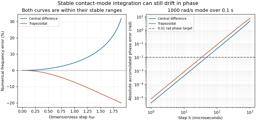
Stable contact-mode timesteps can accumulate substantial numerical phase error
. Exact frequency errors for central differences and the trapezoidal rule, and the resulting absolute phase errors for a fixed 1000 rad/s mode integrated over 0.1 s. The horizontal line is an illustrative 0.01 rad phase budget. These are analytical linear-mode predictions, not contact measurements. Details.
In a contact experiment or simulation, a shifted oscillation phase changes when force maxima and gap crossings are predicted. Damping, changing tangent stiffness and a contact opening can invalidate the fixed-frequency model, so the phase estimate is not by itself an event-time error certificate. A proposed convergence check compares force histories, dominant frequency and event times at successively halved steps, while keeping contact geometry and constitutive parameters fixed. Agreement in maximum penetration alone can miss a phase error that accumulates over many cycles.
Accumulated contact-mode phase drift is the phase difference that builds over many timesteps when a numerical contact mode oscillates at a slightly incorrect frequency. A small error per step can matter after many cycles even when the amplitude remains bounded. The fast oscillations arise naturally in stiff compliant-contact models, whose numerical integration difficulty is described in the primary multibody notes.[ref]
For a fixed undamped mode of angular frequency , step , and numerical phase advance per step, after steps the unwrapped phase error isUnwrapped phase counts complete cycles; reducing it modulo would hide a missed or added cycle. This expression assumes the same fixed mode and a uniform step throughout the comparison.
For central differences, on . Expanding givesFor the trapezoidal rule, instead givesBoth are second-order phase errors at fixed duration, but their signs and leading coefficients differ. Halving approximately quarters the accumulated phase error; doubling the simulated duration approximately doubles it when the mode remains unchanged.
For an original example, choose , and , so and . Central differences give and a phase lead about , or . The relative frequency error is only about , yet the phase lead has become readily visible. The leading-order estimate is .
An approximate phase budget for central differences suggestsWith the preceding mode and duration and , it gives . Taking gives an exact phase lead about . This is far below the oscillator stability boundary; contact-mode timestep stability and timing accuracy impose different requirements.
The associated timing shift is approximately for a fixed phase feature of a nearly sinusoidal mode with small drift. It is not a general contact-event error bound: a changing amplitude, a grazing zero, changing tangent stiffness or an active-contact transition can invalidate that approximation. A variable-step method also needs its actual update analysis; summing uniform-step formulas without checking how successive maps compose is not automatically exact.
A proposed convergence test records a small compressed-contact oscillation over a stated duration, compares unwrapped numerical and reference phases, and repeats with half the step and twice the duration. Compare the force waveform and event times as well as the maximum penetration. Material damping changes the physical response, while numerical phase drift changes the timing of that modeled response; they should be tested separately.
Articles by others on the same topic
There are currently no matching articles.