Contact mechanics studies how touching bodies deform, transmit forces and separate. Even a ball that appears to touch a flat surface at one point develops a finite contact patch: local elastic deformation spreads the load into a nonuniform pressure distribution. Hertzian contact is a useful ideal model when the surfaces are smooth, the contact patch is small and adhesion and friction can be neglected.
The contact patch is part of the solution, rather than a prescribed loaded area. In nonadhesive contact the nonpenetration constraint prevents overlap, and the normal contact force can push but cannot pull; unilateral contact complementarity joins those requirements. Pressing a spherical probe into a specimen while recording force and indentation tests the contact law and can determine a reduced elastic modulus. Surface roughness, plastic deformation and adhesion require additional modeling, especially when interpreting a measured pull-off force.
The center of pressure summarizes where a distributed normal pressure acts. On a planar contact region in , take a nonnegative pressure field and positive total normal force . Its center of pressure is the pressure-weighted positionIt is a continuous weighted mean, rather than necessarily the point of largest pressure. For discrete normal forces at , replace the integrals by sums. The resulting convex combination places the center of pressure inside the contacts' convex hull, or support polygon.[ref]
Underactuated Robotics by Russ Tedrake. Highly-articulated Legged Robots, Center of pressure (CoP) and Zero-moment point (ZMP), The special case of flat terrain
This definition preserves the torque as well as the resultant normal force. About the origin in the contact plane,A single vertical force applied at gives the same torque. Thus its line of action passes through the center of pressure. Conversely, force-and-torque measurements reconstruct the point throughThe origin and sign convention are part of these equations; moving the moment reference above the contact plane requires the corresponding torque translation.
For an original discrete example, four vertical reactions of , , and act at the successive corners , , and in metres. Their total normal force is , with and . Hence the center of pressure is . A rigid plate on four load cells provides a simple force platform implementation: calibrate the force channels and positions, then test known vertical loads at known locations. Subtracting the unloaded plate's own force and moment removes its contribution when reconstructing the added load. This is a proposed measurement test, not experimental data.
A continuous example shows the inverse problem hidden by this useful compression. On a rectangle of length and width , put and choose profiles independent of :Both profiles are positive on . The added polynomial has zero integral and zero first weighted integral:Thus both profiles give and the same center of pressure , while their peak pressures are and . These are pressure distributions with identical resultant force and center of pressure. For , and , both give despite different local loads. A force platform alone therefore does not identify every local pressure.
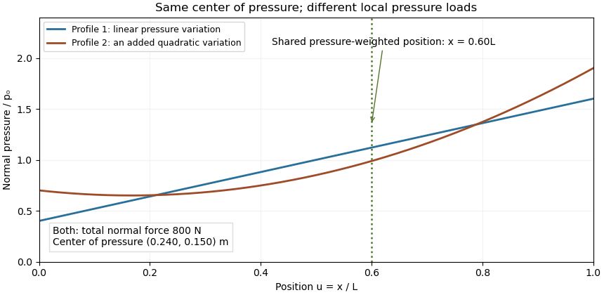
Two limits matter. If , the normal-pressure center of pressure is undefined. At fixed , an absolute moment error changes the reconstructed by , so fixed absolute measurement uncertainty is amplified as a contact unloads. Also, tangential contact forces can leave a residual contact torque at the center of pressure: with full resultant ,Selecting the normal-pressure centroid does not force this yaw torque to vanish.
Under the gravity-only, resting assumptions of support polygon, the center of pressure coincides with the horizontal center of mass projection. During motion it need not. For a planar model driven only by gravity and ground contact forces, at fixed center of mass height and with constant angular momentum about that centre, force and torque balance give . The acceleration term explains why the center of pressure is a contact-force measurement rather than a general substitute for center of mass position.[ref]
Underactuated Robotics by Russ Tedrake. Highly-articulated Legged Robots, equations cop and zmp and their stated constant-height/angular-momentum assumptions
In terrestrial robot locomotion, the center of pressure is the ground point summarizing the normal load shared by the active contacts. With contact positions and nonnegative normal reactions , its coordinates are the weighted averages and , provided the total normal force is positive. It lies in the current support polygon, but is a contact-force quantity rather than the robot's center of mass position.[ref]
Underactuated Robotics by Russ Tedrake. Highly-articulated Legged Robots, Center of pressure (CoP) and Zero-moment point (ZMP), flat-terrain definition
Force-sensor coordinates matter when reconstructing this point. Suppose a sensor origin lies height above a horizontal contact plane, with parallel coordinate axes. If it reports force and moment , the plane point is located at relative to that origin. Moment translation givesThe ground-plane transformation of a measured contact wrench must therefore precede interpreting moment/force ratios as a contact location.
For an original sensor example, take , force , and measured roll/pitch moments . The reconstructed point is . Ignoring the origin height would instead give . Those millimetre differences are coordinate effects, not a change in the physical pressure distribution.
During motion, the contact point need not equal the horizontal projection of the center of mass. The source's constant-height, negligible-angular-momentum-rate model relates their difference to horizontal acceleration; those assumptions must be established before using that simplified relation.[ref] A robot-foot experiment can compare known applied loads with the sensor's translated force/moment measurements. When approaches zero, reconstruction becomes sensitive to moment error; at zero normal load the normal-pressure point is undefined. A residual yaw couple may remain, as explained in residual contact torque at the center of pressure.
A ground-plane transformation of a measured contact wrench combines a change of coordinate axes with a change of the point about which moments are reported. A six-component wrench is incomplete without both pieces of metadata. Drake's primary SpatialForce reference explicitly tracks the application point and expressed-in frame separately from the stored force and torque values.[ref]
SpatialForce class in Drake documentation. Detailed Description; Shift and ShiftInPlace
Let rotate sensor-frame components into ground-frame components, and let be the ground-frame vector from ground origin to sensor origin . For measured force and moment about , the equivalent result about isThe plus sign uses the stated vector from the new origin to the old one. A shift expressed with the opposite vector uses the opposite sign. The offset and force must be expressed in the same axes before taking the cross product.
For a planar normal-pressure reconstruction with , computeThe special parallel-axis height correction in center of pressure is recovered with and .
For an original rotated-sensor example, use a 90-degree rotation about , sensor readings and , and . Rotation gives and . The translated moment is , yielding . The yaw moment remaining at that point is , so translating to the centroid does not erase the entire wrench.
A bench check applies known loads at known ground locations and repeats after changing sensor orientation. Geometry, tare loads, units and axis signs must all be included. A correct rotation with the wrong moment origin can still give an incorrect pressure location; a small normal load also amplifies reconstruction uncertainty.
The center of pressure locates the resultant of a distributed fluid pressure load relative to its moment. On a planar surface carrying parallel pressure forces, the first-moment ratio in center of pressure applies. On an airfoil, pressure variation and its resultant can change with the flow state, so the point is not a permanently fixed geometric centre. NASA's primary account explicitly distinguishes a moving center of pressure from retaining a force and pitching moment about an aerodynamic center.[ref]
Center of Pressure by NASA Glenn Research Center. Center of Pressure, Angle of Attack, and Aerodynamic Force sections
For an original hydrostatic plate example, take a vertical rectangle of width , extending from the free surface to depth in a constant-density fluid. If the same atmospheric pressure acts on its other face, the net gauge pressure at depth is . This hydrostatic relation follows from vertical force balance.[ref]
The Feynman Lectures on Physics, Volume II by Richard Feynman and others. Chapter 40, §40–1, Hydrostatics
The resultant and its depth areFor , , and , the net force is at depth . The area centroid is only one metre below the surface; the increasing pressure shifts the load's centroid downward.A tank demonstration can infer the resultant line from the force and hinge moment on a small plate while changing the water depth. The plate's own gravitational moment and the pressure on both faces must be included. This tests a specified pressure-load model, not a general claim that the point always lies below every geometric centre.
For aerodynamic net loads, differences of pressures on opposite faces can have both signs. The convex-hull property proved for nonnegative contact pressure then need not apply, and a small resultant with a finite moment makes its location ill-conditioned. A curved surface or a general wrench may also require a residual couple rather than a single force that removes every component of torque. The resultant convention and moment reference are therefore part of the definition.
A residual contact torque at the center of pressure is the moment left after translating a planar contact's resultant force to its normal-pressure centroid. Let the resultant wrench at an origin in be force and moment , with . Put , where and . Translation givesThe two horizontal moment components vanish, but the yaw component need not. The zero-moment-point construction for flat robot contact removes moments perpendicular to the surface normal; it does not assert that every component is zero.[ref]
Underactuated Robotics by Russ Tedrake. Highly-articulated Legged Robots, An aside: Zero-moment point derivation
A useful invariant makes the limitation exact. Since ,If this scalar is nonzero, no change of the moment origin can eliminate the entire moment vector. Replacing the whole contact by only one force at the center of pressure would discard that information.
For an original two-contact example, put equal normal loads of at and metres. Add tangential forces at the positive position and at the negative position. The total force is , the pressure centroid is the origin, and the opposing tangential forces give a pure yaw couple of . A friction coefficient of at least permits the stipulated tangential magnitudes at these loads.
A normal-load-only reconstruction would identify the correct centroid while missing the couple. A sensor measuring all force and moment components can distinguish the two situations. The origin, surface orientation and axis signs must be retained when comparing measurements. Near zero normal load, the centroid reconstruction itself becomes singular, independently of whether a tangential moment remains.
Pressure distributions with identical resultant force and center of pressure demonstrate that a pressure centroid is not a reconstruction of a pressure field. A normal-load measurement and its two first spatial moments constrain onlyA perturbation preserving all three integrals leaves the resultant and center of pressure unchanged. It is physically admissible only when the perturbed field remains nonnegative under the nonadhesive pressure model. The polynomial profiles in the parent article give one smooth example; the following construction shows that even a peak-pressure bound is missing.
Take a rectangular region of length and width , centered about its midpoint, and fix a normal load . A uniform field has pressure and centroid . Instead place the entire load uniformly on a smaller centered square of side , with zero pressure outside that square. Its pressure isSymmetry fixes the same centroid, and integration still gives total force . Yet its peak is , which has no upper bound as shrinks. Smooth symmetric concentrated profiles can provide the same conclusion if a continuous pressure field is required.
For an original numerical example, let , , and . Uniform pressure is . Concentrating the same load on a centered square gives while preserving the measured point . Both satisfy the stated nonnegative-field moment constraints.
Consequently a force/moment sensor cannot infer local peaks from the centroid alone. Local contact pressure from additional spatial measurements needs more data or justified material/contact assumptions, such as a constitutive model and known geometry. The source's normal-force centroid definition explains exactly which resultant information was retained.[ref]
Underactuated Robotics by Russ Tedrake. Highly-articulated Legged Robots, Center of pressure definition
The examples are inverse-problem constructions; they are not claims that arbitrary pressure maps can be realized by the same elastic surfaces.Local contact pressure from additional spatial measurements requires more information than total normal force and two first moments. One explicit reconstruction model partitions the contact into cells of known areas and centroids , assuming uniform pressure within each cell. Writing givesThese are three linear measurements of the cell loads. They need not determine every , as the nonuniqueness argument in pressure distributions with identical resultant force and center of pressure shows. The primary centroid definition specifies precisely which force/moment information is retained.[ref]
Underactuated Robotics by Russ Tedrake. Highly-articulated Legged Robots, Center of pressure definition
For an original four-cell example, use equal cells centered at successive positions with . Loads give and centroid . Adding to these loads changes neither the sum nor either first moment. Nonnegative loads permit . The alternative therefore gives the same global measurements.
An independently calibrated measurement of the first cell load resolves this one missing degree of freedom under the four-cell model. If it reads , the global moment equations recover the original other three loads. Their cell pressures are . Measuring all four cells instead provides redundant data for checking total load and the assumed geometry.
The local sensor output must actually represent a known cell-integrated force, or have a validated response model; a point sample cannot automatically be treated as an area average. Calibration errors, cell cross-coupling and imperfect coverage become additional measurement inputs. Spatial pressure-map resolution below a sensor cell remains limited even when every cell average is known: unmeasured within-cell peaks are not recovered by simply drawing a finer image. Constitutive or smoothness assumptions can add information, but must be identified as assumptions rather than extra measurements.
Spatial pressure-map resolution below a sensor cell concerns which variations of a contact pressure field can actually be distinguished by spatial measurements. A smaller display pixel does not imply a smaller independently measured contact region. The response of a pressure sensor, its sampling positions and any imposed reconstruction assumptions must be specified.
For an original ideal array model, cell of known area reports an area-average pressure,It determines that cell’s load , but not every value inside it. For a more general linear response, with known sensitivity . The null space of a spatial pressure measurement consists of perturbations whose weighted integrals vanish for all measured channels. Nonnegative fields that differ by such a perturbation remain indistinguishable in that model.
Consider square cells of side aligned with , and compare fields independent of :Every cell contains one full cosine period, so both fields give every channel the identical value . Yet varies between and . With and , a perfectly uniform field and a field spanning – produce the same ideal map. On an aligned finite rectangular array, the added cosine also has zero first moment within each cell, so even the global resultant and center of pressure agree. This is an inverse-problem construction, not a claim that both profiles arise from the same elastic contact geometry.
Cell averaging has a calculable spatial response. For a one-dimensional centered interval of width , averaging a complex wave multiplies its value at the interval center byThe first zero at explains the erased cosine above. Sampling introduces further ambiguity; even translating this ideal array cannot recover a component erased by its aperture at every position.
A regularity assumption can supply a conditional bound. If has a validated spatial Lipschitz constant over a square cell, its center value differs from its area average by at mostEvery point in the cell is at most half the diagonal from its center, so integrating the Lipschitz inequality proves this bound. For and , it gives about . The array readings alone do not establish that slope bound.
Interpolation chooses a finer representation from the measured values. SciPy explicitly describes its array zoom operation as spline interpolation; it does not describe collecting new pressure data.[ref] A proposed apparatus test scans a known small indenter across a sensor array at controlled total load, comparing independent load measurements with channel responses. The indenter’s actual contact area, load spreading, sensor cross-coupling and repeatability must be measured before inferring a spatial response. Additional smaller-aperture measurements or justified mechanical constraints can improve identifiability; a smoother image alone supplies neither.
The null space of a spatial pressure measurement consists of changes to a contact pressure field that leave every measured channel unchanged. For a linear response model on a contact region , writeThen . Two fields have identical outputs precisely when their difference lies in this kernel of a linear map. The sensitivity kernels , their support and the admissible class of pressure fields are part of the model.
For an ideal area-average sensor, inside cell and zero elsewhere. A positive and negative perturbation within one cell can cancel in its integral while remaining invisible to the other cells. This is the mechanism behind spatial pressure-map resolution below a sensor cell. It is a nonuniqueness of the observations, even if their numerical values are exact.
An original finite model divides each of two equal-area sensor cells into two equal halves with constant pressures . The observed averages areThis matrix has rank two and a two-dimensional null space spanned by and . Thus the fieldsboth produce . Their peak pressures differ by . Adding an independent measurement of determines the first pair, but still leaves the second pair’s difference undetermined. An extra channel helps only if it adds an independent constraint on the missing directions.
The linear null space is not itself a set of physical pressure fields: its perturbations can have either sign. For a nonadhesive contact, require as well. With the uniform field above, perturbations are admissible for . Positivity restricts the ambiguity without removing it. In contrast, a zero area-average reading together with a nonnegative pressure assumption forces pressure to vanish almost everywhere in that cell under the ideal model.
For a chosen finite basis of pressure fields, a singular value decomposition identifies the matrix null space. SciPy’s pinned implementation constructs its basis from right singular vectors and uses a relative singular-value cutoff to determine effective numerical rank.[ref]
SciPy 1.16.2 documentation. scipy.linalg.null_space, pinned v1.16.2 scipy/linalg/_decomp_svd.py, docstring and implementation lines 333–403
A numerical cutoff and an exact zero singular value are different notions. Near-null directions of a pressure sensor array have small nonzero responses and can amplify measurement error: a dimensionless singular value of turns a channel-error component into a coefficient error when inverted without regularization.A proposed apparatus check applies controlled local loads to estimate the sensitivity kernels, then compares fields with similar predicted channel outputs using independent spatial measurements. Contact area, load spreading and cross-coupling must enter that comparison. A reconstruction algorithm may select one smooth or nonnegative solution, but the selected structure is additional modeling information; it is not automatically an independently observed subcell pressure map.
Near-null directions of a pressure sensor array are changes of a modeled pressure field that produce small, rather than exactly zero, changes in the sensor outputs. They distinguish an ill-conditioned reconstruction from the exact ambiguity in the null space of a spatial pressure measurement. A formally invertible response can still contain very little usable information about some pressure patterns.
Choose a finite basis for the pressure field and a linear response , where contains pressure coefficients, the readings, and measurement error. With common pressure units for the coefficients and readings, letbe a singular value decomposition. A change changes the noiseless readings by . Inverting that component divides the measurement error by . If the errors have covariance , the standard deviation of the reconstructed coefficient along is . An exact zero gives no inverse; a small nonzero value gives noise amplification.
An original two-region example has uniform pressures and sensor matrixBoth sensors mostly measure the same average. Write and . Then and . Uniform pressures give readings ; the markedly different pair gives only . The matrix is invertible, but these outputs differ by just in one channel.
If each channel has independent standard uncertainty, the direct contrast estimate is , with standard deviation about . The matrix’s smallest singular value is approximately , consistent with roughly uncertainty in the unit-length contrast direction. Nonnegative pressure constraints can restrict the admissible answers, but do not turn these noisy readings into precise contrast information.
Numerical rank depends on a chosen tolerance. SciPy’s pinned null-space implementation compares singular values with a relative cutoff and returns right singular vectors beyond the retained rank.[ref]
SciPy 1.16.2 documentation. v1.16.2 scipy/linalg/_decomp_svd.py, null_space, docstring and lines 395–403
A floating-point cutoff detects numerical scale; a physical decision about usable information must also consider sensor noise, response uncertainty and the chosen pressure basis. Rescaling a coefficient can change a raw singular value without changing the apparatus.A noise-whitened pressure sensing matrix accounts for unequal or correlated measurement errors before comparing response strength. For positive-definite error covariance , analyze together with the same coefficient units and normalization. A duplicate noisy channel does not provide the same information as an independent measurement of the weak contrast.
Tikhonov regularization can limit amplification by using factors instead of . Relative to the true noiseless coefficient, this introduces attenuation . For and , that factor is about : the weak component is nearly suppressed. A smoother map can therefore have less noise while omitting real contrast. A proposed validation applies independently known pressure patterns that excite both average and contrast directions, repeats the measurements, and reports the error covariance and response-model uncertainty alongside reconstruction results.
A noise-whitened pressure sensing matrix measures how a contact pressure pattern changes sensor outputs relative to their joint noise, rather than their raw numerical size. For a linear measurement modelassume the error covariance is positive definite. Choose an invertible matrix satisfying . ThenThe transformed errors have identity covariance. This is the whitening transformation documented in the primary SciPy covariance interface; its example obtains approximately identity sample covariance from simulated observations.[ref]
A Cholesky decomposition supplies . Compute and by solving triangular systems rather than forming an inverse unnecessarily. The least-squares residual becomesThus an output change is significant according to its noise covariance, not merely the Euclidean length of the raw readings. The original pressure basis and its units must still be stated; whitening rows does not remove arbitrary column rescalings.
For an original two-channel example, use numerical pressure values in kilopascals andThe separate standard deviations are and with correlation . A residual whitens to , giving squared length about . The residual instead whitens to , giving squared length . Treating the channels as independent would assign both residuals squared standardized length two. The positively correlated noise makes opposite-sign discrepancies much less plausible than a shared shift.
A simple repeated-measurement model illustrates the information consequence. If two sensors measure the same scalar pressure with equal standard deviation and correlation , their mean has variance . At the standard deviation is about , rather than the independent-channel value . Adding an almost duplicate channel therefore supplies little improvement for that common pressure.
The pressure-map information matrix is . In a full-column-rank linear Gaussian model with known , the unconstrained weighted least-squares estimate has covariance . Small singular values of identify near-null directions of a pressure sensor array after accounting for noise. Alternative whiteners differ by an orthogonal row transformation and give the same information matrix; an individual whitened row need not represent one physical sensing cell.
A proposed array characterization applies repeatable known pressure patterns, estimates the channel covariance from repeated residuals, and checks the covariance on independent repeats after whitening. Drift and response-model uncertainty must be included if they belong to the intended error model. If is singular, a simple inverse whitening is unavailable: exact zero-noise constraints and redundant stochastic directions need separate treatment. A visually smooth pressure reconstruction does not establish that its weak directions were measured precisely.
A pressure-map information matrix quantifies which coefficients of a modeled contact pressure field are constrained by a sensor array, relative to its measurement noise. For with fixed positive-definite error covariance , defineHere is the noise-whitened pressure sensing matrix. Whitening removes the output-noise covariance from the residual metric; the primary SciPy covariance interface documents this transformation and demonstrates near-identity covariance on simulated observations.[ref]
The matrix is positive semidefinite because . Its null space is exactly the null space of : an unobserved pressure change remains unobserved after invertible row whitening. With independent Gaussian errors of known covariance, the log likelihood is a constant minus . Differentiating twice with respect to gives negative Hessian , identifying it as the Fisher information for this stated model.
If has full column rank, weighted least squares givesThis covariance follows by substituting and multiplying the error matrices. It concerns the unconstrained linear estimator with known response and covariance, not every reconstruction algorithm. Nonnegativity constraints, regularization and uncertain sensitivity kernels require additional treatment.
An original two-cell example begins with one average-pressure measurement, , with standard error. In numerical kilopascal coordinates,Its eigenvalues are and zero: the mean is observed, but the pressure difference is not. A second independent copy doubles the information matrix while leaving the difference unobserved. More repeats of the same mixture improve precision only in the already measured direction.
Instead add a direct measurement of the first cell with the same independent error. NowThe inferred first-cell pressure has standard deviation and the second . Their errors are negatively correlated because the second pressure is reconstructed by subtracting the first from twice the measured mean.
A rank-one update of pressure-map information follows when an independent new channel has sensitivity row and error variance : its added information is . A channel aligned with a weak pressure direction can therefore be more useful than another precise copy of a strong direction. Correlated new errors cannot be added by that independent-channel formula.
A proposed characterization uses repeatable known loading patterns to estimate , independent repeats to estimate , and withheld patterns to test predicted reconstruction covariance. State the pressure basis and units: rescaling a coefficient changes the numerical information entries. A sharp reconstructed image or a large matrix determinant alone does not establish that the underlying response model or noise assumptions are correct.
A rank-one update of pressure-map information describes the extra constraint supplied by one independent scalar pressure measurement. Suppose the existing pressure-map information matrix is , and a new sensor reports with known variance , independent of the existing errors. Adding its squared residual to the weighted least squares objective givesThe added matrix has rank one when . It is positive semidefinite because its quadratic form is . Thus the new observation cannot reduce information in any direction under this fixed linear map and noise model. The noise normalization is the same whitening transformation used to express a correlated residual metric as an ordinary squared norm.[ref]
The update can remove a missing direction only if the new channel actually sees it. More precisely,This follows because a sum of two nonnegative quadratic forms is zero exactly when both are zero. Repeating an existing mixture improves its precision but cannot identify a pressure contrast that all mixtures annihilate.
When is positive definite, write . The Sherman–Morrison formula yields the updated estimator covariance matrixMultiplication by verifies the identity directly. For a particular quantity , its variance falls by . A small noise level is valuable only together with a useful sensitivity direction.
For an original calculation in kilopascal coordinates, let , and . ThenThe variance of the sum drops from to . The negative off-diagonal entry means the two inferred coefficients now have negatively correlated errors; it does not mean either individual variance is negative.
A correlated-channel update of pressure-map information needs the new channel's residual after predicting it from old channel noise. Simply adding double-counts information when a common amplifier or reference contributes correlated errors. A proposed array experiment uses repeated known loads to estimate sensitivity and noise separately, adds one channel, and compares withheld-load errors with . Agreement tests the full assumed model, including independence and unchanged sensor response, rather than the matrix identity alone.
Unilateral contact permits bodies to separate while preventing them from passing through each other. In an ideal rigid, nonadhesive model, the supporting normal contact force can push but cannot pull. It is therefore different from a permanently attached support: an upward pull may lift a body away instead of producing a downward support reaction.
Let be the signed normal gap, positive when the bodies are separated, and the outward compressive normal contact force. The nonpenetration constraint and absence of adhesion give the unilateral contact complementarity conditionsAn open gap requires , while requires a closed gap. The pair is also allowed: touching does not by itself imply a loaded contact.[ref]
Underactuated Robotics by Russ Tedrake. Multi-Body Dynamics, Time-stepping LCP: Normal force, nonnegative gap and normal reaction and their complementarity product
Tangential friction requires an additional relation such as Coulomb friction; it is not specified by the normal-gap conditions.The equation of motion is still needed to determine the reaction. Consider a block of mass on a fixed horizontal floor, initially at rest at , with an upward applied force through its center of mass. With upward positive, Newton's second law isIf the contact remains closed, would require . That is feasible for . For , a negative normal reaction would violate unilateral contact, so the contact opens with and . At a closed contact with zero normal velocity, the appropriate acceleration-level contact complementarity iswhich yieldsThese acceleration conditions are being applied at a closed, initially stationary contact; they are not a rule forbidding downward acceleration during separated free flight.
For an original numerical example, let and . Pulling upward with leaves a normal reaction of . At , the reaction is zero and the initial upward acceleration is . At , both the reaction and the initial acceleration vanish, while touching remains possible.
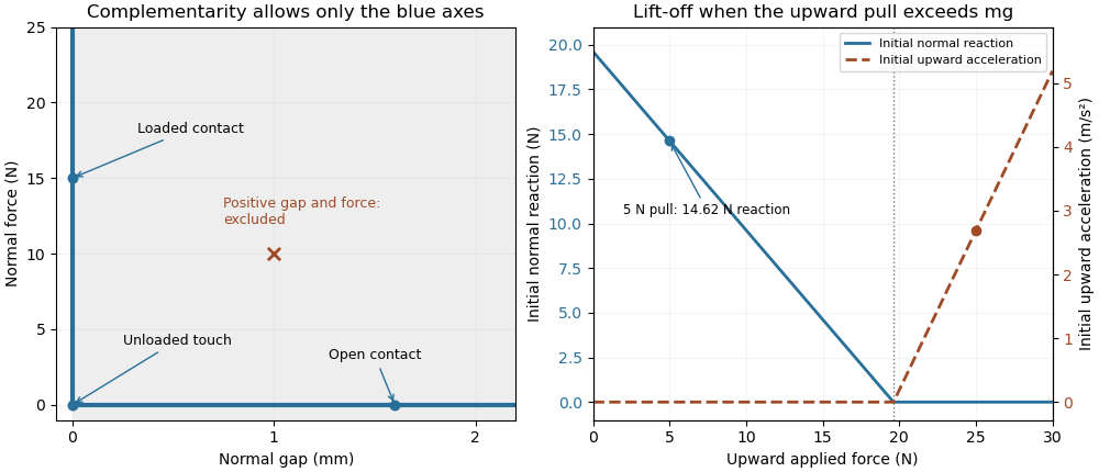
Unilateral contact allows a closed unloaded contact and releases a support when a tensile reaction would be required
. Original ideal-model illustration. The left panel shows allowed gap/reaction pairs; the right shows the initial reaction and acceleration for a stationary 2 kg block as an upward pull is increased. The two panels illustrate geometry and force balance respectively; they are not measured loading data. Details.A simple apparatus test places the block on a calibrated load cell and applies the upward pull through a spring balance, keeping the pull vertical through the center of mass to avoid an extra overturning torque. The support reading should decrease with the pull while contact persists, then vanish at lift-off. Recording the gap as well distinguishes an unloaded touch from a genuinely open contact. Real support elastic deformation and adhesion must be accounted for before treating that apparatus as the ideal rigid, nonadhesive model.
A penalty approximation of unilateral contact replaces perfect rigidity by a chosen stiff response, for exampleHere a small negative gap represents an allowed modeled overlap relative to undeformed reference surfaces. It is not an exact solution of . For the supported load above and chosen penalty stiffness , equilibrium requires . Increasing reduces that overlap at the same load. The penalty method and the ideal constraint are different approximations of the contact response.
Finally, impact requires a rule for the velocity change. The position-level inequalities alone do not decide whether an approaching body sticks or rebounds. A coefficient of restitution or another specified impact law determines that behavior, and the impulsive contact force is summarized by its impulse. Tedrake's particular time-stepping formulation identifies its block collisions as perfectly inelastic; that is a feature of the stated model, not a consequence of the three gap/reaction inequalities alone.[ref]
Underactuated Robotics by Russ Tedrake. Multi-Body Dynamics, Time-stepping LCP dynamics for block collision, perfectly inelastic collision hint
A penalty approximation of unilateral contact allows a small modeled overlap and uses a stiff restoring force instead of enforcing an exact rigid nonpenetration constraint. With signed gap , positive in separation, a simple nonadhesive law isAn open or just-touching contact has zero force in this spring law; a sustained compressive load requires negative . Thus it approximates unilateral contact rather than satisfying its rigid gap condition exactly. Tedrake's primary compliant-contact treatment uses stiff springs and damping to resist penetration and explains the resulting numerical stiffness.[ref]
For an original gravity-supported example, a mass with no other vertical load has . With , its static overlap is . Increasing by a factor of 100 reduces that overlap to , but also makes the contact dynamics faster.
While the contact stays compressed, linearization about equilibrium givesThe normal contact penalty time scale is therefore proportional to . For the first stiffness above, ; after increasing stiffness it is ten times larger. At fixed numerical step size, a smaller overlap error need not mean a more accurate trajectory.
For example, the Forward Euler method applied to this undamped oscillator has amplification factors , whose magnitudes exceed one for every positive step. Merely shrinking the step does not make that method asymptotically stable for indefinite undamped oscillation, although it can reduce error on a finite interval. A suitable integration method, damping model and convergence check must be chosen. The source notes specifically identify stiff differential equations as a challenge for compliant contact simulation.[ref]
Underactuated Robotics by Russ Tedrake. Multi-Body Dynamics, Compliant Contact Models, numerical integration discussion
A penalty stiffness is a chosen model parameter, not automatically the actual material stiffness. Impact dissipation and tangential friction still need their own constitutive choices; a purely elastic normal spring does not imply a perfectly inelastic collision.
The normal contact penalty time scale describes the fast dynamics introduced by a stiff normal-contact approximation. For a compressed linear penalty spring with stiffness acting on a point mass , small oscillations about equilibrium satisfy . Their angular frequency, reference time and period areThe reference time is not the full oscillation period. Rescaling time by gives , so a numerical step is controlled by its dimensionless size , not just its duration in seconds. The primary compliant-contact treatment highlights the numerical stiffness caused by such springs.[ref]
A modeling and numerical budget interact. Limiting equilibrium overlap under a specified maximum supported load to requires in this linear model. For an original choice and , choose . At ,A chosen resolution target of twenty steps per contact oscillation would set . This is a resolution target, not a universal accuracy or stability theorem for every integrator.
Increasing the stiffness by a factor of 100 reduces the same-load overlap by 100 but reduces these times by only ten. Keeping the old step then gives roughly two samples per new oscillation instead of twenty. The parent penalty approximation of unilateral contact also shows why the Forward Euler method's undamped-oscillator instability cannot be cured merely by calling the step small.
For a multibody contact, the effective mass in a normal-contact penalty mode replaces an arbitrary total body mass. Additional damping and nonlinear force laws can introduce other time scales. A convergence study should therefore check force histories and contact events as well as maximum overlap; smaller geometric penetration alone does not establish a more accurate simulation.
The effective mass in a normal-contact penalty mode is the inertia seen by one specified relative normal displacement, rather than automatically the total mass of either body. A contact away from a center of mass can excite rotation as well as translation, changing that inertia and the normal contact penalty time scale.
Use independent generalized velocities , a positive-definite mass matrix , and a normal gap whose local velocity is . A scalar normal force produces generalized force . The primary multibody formulation gives this contact-Jacobian velocity/force pairing explicitly.[ref]
Underactuated Robotics by Russ Tedrake. Multi-Body Dynamics, Contact modeling: contact Jacobian and equation with generalized force J-transpose times lambda
At a frozen configuration, the part of gap acceleration caused by that force isIf the scalar is positive, defineThe definition uses a physical normal gap measured in metres and a matching normal force measured in newtons. Arbitrarily rescaling the gap coordinate changes the associated inertia. Constraints must first be accounted for by independent coordinates or the appropriate constrained response.A short normal impulse gives , hence . This supplies a direct interpretation: less effective mass means a larger relative normal-velocity change for the same impulse. At a fixed local configuration, a compressed linear penalty spring of stiffness gives the small-motion estimateIt omits changing contact geometry, other driving forces and damping; the source separately explains why stiff compliant contact challenges numerical integration.[ref]
For two freely translating particles, the relative gap sees , so . This is the reduced mass. Equal particles give ; replacing one by a fixed wall gives instead.
For a planar rigid body above a fixed plane, let its mass be , rotational moment of inertia about its center be , and the contact normal be vertical. A contact a horizontal distance from the center hasFor , and , . At the center it is . With , the off-center angular frequency is , compared with at the center. Using the full mass in both cases misses this rotational response.
Several simultaneous contacts require more than separate scalar replacements. Their matrix generally has off-diagonal terms: a force at one contact changes another contact’s acceleration. With frozen geometry and positive diagonal stiffness matrix , compressed gap perturbations satisfy ; its nonzero modal squared frequencies are those of the symmetric matrix . Coupled normal-contact penalty modes can therefore be faster than estimates treating each contact independently. A proposed verification applies a small known impulse or displacement perturbation at a stated configuration and checks relative contact motion, followed by a timestep convergence study.
Coupled normal-contact penalty modes are small oscillations generated by several simultaneously compressed penalty contacts acting through shared body inertia. A displacement at one contact can accelerate another because both load the same translating or rotating bodies. Separate scalar effective mass in a normal-contact penalty mode estimates do not generally give the coupled frequencies.
Freeze a contact configuration, use independent generalized displacement perturbations , positive-definite mass matrix , and gap perturbations . Let be a positive diagonal matrix of normal penalty stiffnesses. After subtracting equilibrium loads, the restoring generalized force is , soThe contact-Jacobian force/velocity pairing and stiff compliant-contact model come from the primary multibody formulation; the local modal reduction here follows by substitution.[ref]
Although need not be symmetric, it is similar to the symmetric positive-semidefinite matrix . Set to obtainIts positive eigenvalues are squared angular frequencies. A zero eigenvalue may describe redundant gap coordinates outside the realizable displacement subspace; it should not automatically be interpreted as an extra physical oscillation. Free generalized motions satisfying are a separate possibility.
For an original planar example, a rigid bar has vertical translation , small rotation , mass , center-of-mass moment of inertia , and two vertical contacts at horizontal offsets . ThenWith equal contact stiffness , the equal-gap mode is vertical translation and the opposite-gap mode is rocking. Their angular frequencies areTake , , and . Then has diagonal entries and off-diagonal entries . Its eigenvalues are and , giving and . Treating the contacts independently would assign each and miss the faster rocking mode.
Contact-mode timestep stability depends on the largest active frequency and on the integrator. For the undamped central-difference recurrence, one mode has amplification equationThe distinct oscillatory roots lie on the unit circle for ; the endpoints need separate treatment. The example therefore requires for this linear stability condition. Resolving the waveform accurately normally requires a smaller step. This is not a stability rule for every integration method.
The derivation applies while both contacts remain compressed and geometry is locally constant. A sufficiently large rocking amplitude can unload one contact, changing the active model. A proposed check preloads both supports, applies small symmetric and antisymmetric perturbations, and compares measured or simulated frequencies with the two predictions. Repeat with smaller amplitudes and smaller timesteps to separate linearization error, contact opening and numerical error.
Contact-mode timestep stability concerns whether a numerical integrator introduces growing errors when advancing the fast dynamics of an active penalty contact. It depends on the integration rule and the local modal frequencies, not just the size of the modeled overlap. The primary compliant-contact treatment identifies stiff contact springs as a source of numerically stiff differential equations.[ref]
Underactuated Robotics by Russ Tedrake. Multi-Body Dynamics, Compliant Contact Models, stiff-spring and numerical integration discussion
Freeze the active contacts and linearize about a compressed equilibrium. An undamped mode has . For step , put . The Forward Euler method updates displacement and velocity with matrixwhose eigenvalues are . Their magnitudes are whenever . Thus the method has no nonzero stable step for indefinite integration of this undamped oscillator, although smaller steps reduce its error on a fixed finite interval.
The central-difference recurrence instead givesFor its two distinct amplification roots lie on the unit circle. At the repeated root is , and solutions can include , so the strict bound matters. A collection of frozen undamped modes therefore requires for this oscillatory stability condition. In coupled normal-contact penalty modes, comes from the coupled system rather than an arbitrary total-mass estimate.
Stability still allows substantial contact-mode numerical phase error. For central differences the phase per step is , giving numerical angular frequency . At and , is stable but the numerical frequency is about , high. A timing-sensitive contact event can consequently drift even when oscillation amplitudes do not grow.
Implicit schemes illustrate another tradeoff. For the Backward Euler method, the amplification factors are and have magnitude . At , each step reduces the oscillatory amplitude by about , despite the continuous undamped system conserving energy. The trapezoidal rule instead has factorswith phase . The same example gives , low. Unconditional stability for this linear model does not imply correct timing at a large step.
A practical error check therefore compares both amplitude and phase while reducing . For instance, a small target dimensionless step gives much smaller phase error than one, but the acceptable value depends on the observable and time span; it is not a universal accuracy certificate.
The frozen-mode argument has a defined scope. Contact opening changes the active stiffness, nonlinear force laws change tangent stiffness, and damping introduces additional eigenvalue scales. An integrator can satisfy the local oscillator bound while missing an intervening collision or contact release. A proposed test starts with a small compressed-contact perturbation, checks frequencies and energy behavior, then repeats across a known contact-opening event with decreasing steps. Record force histories and event times as well as penetration, so numerical damping or phase drift is not mistaken for a material response.
Contact-mode numerical phase error is the difference between the oscillation phase produced by a time integrator and the phase of the modeled contact dynamics. It can grow while the numerical solution remains bounded. Contact-mode timestep stability controls a different property; stable integration alone does not ensure accurate force timing or contact-event timing. The physical motivation is the fast oscillation introduced by a stiff compliant contact model.[ref]
Underactuated Robotics by Russ Tedrake. Multi-Body Dynamics, Compliant Contact Models, stiff-spring and numerical integration discussion
For a frozen undamped contact mode , central differences givePut and use . On the stable branch ,The numerical frequency exceeds the modeled frequency. A Taylor series givesFor the trapezoidal rule, its amplification-factor phase instead givesThat scheme preserves modal amplitude in this undamped linear setting while lagging in phase. These formulas isolate a single mode with fixed frequency and consistent initialization; general nonlinear contacts require additional analysis.
Accumulated contact-mode phase drift after a duration is at time-grid points. For an original example, let and . With , the central-difference frequency is about , producing of phase lead. The step satisfies the strict stability inequality, yet the phase lead exceeds half a cycle.
Reducing to gives about of lead over the same duration. At it is about , approximately one quarter as large, matching the leading second-order error. For a small desired phase budget , the central-difference expansion suggestsWith , this estimate is about , much smaller than the stability boundary. Check the exact frequency formula when the small-step expansion is not sufficiently accurate.
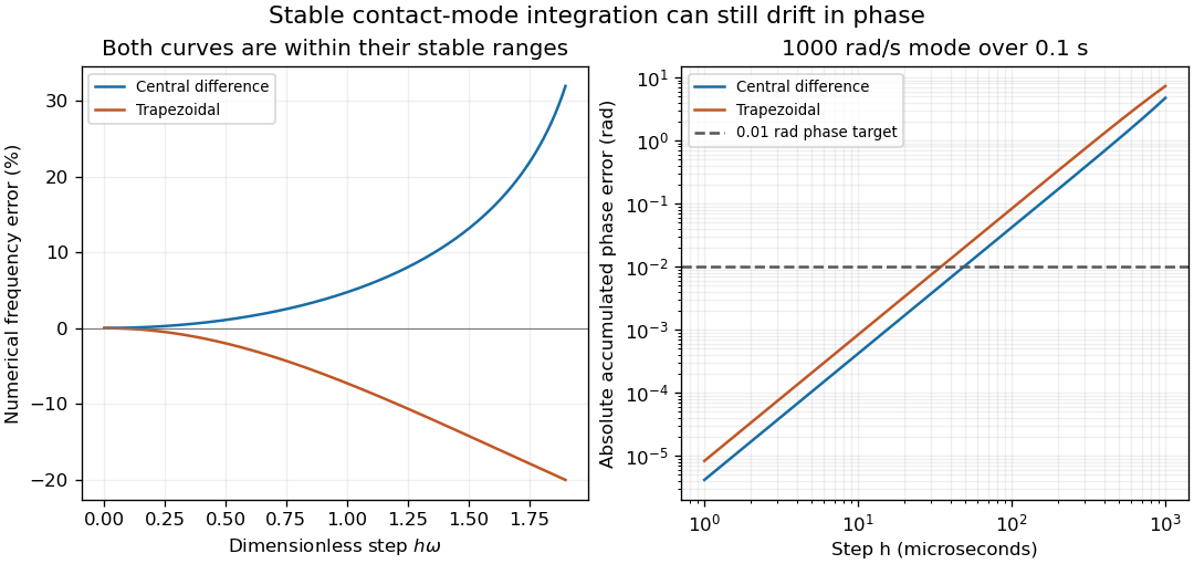
Stable contact-mode timesteps can accumulate substantial numerical phase error
. Exact frequency errors for central differences and the trapezoidal rule, and the resulting absolute phase errors for a fixed 1000 rad/s mode integrated over 0.1 s. The horizontal line is an illustrative 0.01 rad phase budget. These are analytical linear-mode predictions, not contact measurements. Details.In a contact experiment or simulation, a shifted oscillation phase changes when force maxima and gap crossings are predicted. Damping, changing tangent stiffness and a contact opening can invalidate the fixed-frequency model, so the phase estimate is not by itself an event-time error certificate. A proposed convergence check compares force histories, dominant frequency and event times at successively halved steps, while keeping contact geometry and constitutive parameters fixed. Agreement in maximum penetration alone can miss a phase error that accumulates over many cycles.
Accumulated contact-mode phase drift is the phase difference that builds over many timesteps when a numerical contact mode oscillates at a slightly incorrect frequency. A small error per step can matter after many cycles even when the amplitude remains bounded. The fast oscillations arise naturally in stiff compliant-contact models, whose numerical integration difficulty is described in the primary multibody notes.[ref]
For a fixed undamped mode of angular frequency , step , and numerical phase advance per step, after steps the unwrapped phase error isUnwrapped phase counts complete cycles; reducing it modulo would hide a missed or added cycle. This expression assumes the same fixed mode and a uniform step throughout the comparison.
For central differences, on . Expanding givesFor the trapezoidal rule, instead givesBoth are second-order phase errors at fixed duration, but their signs and leading coefficients differ. Halving approximately quarters the accumulated phase error; doubling the simulated duration approximately doubles it when the mode remains unchanged.
For an original example, choose , and , so and . Central differences give and a phase lead about , or . The relative frequency error is only about , yet the phase lead has become readily visible. The leading-order estimate is .
An approximate phase budget for central differences suggestsWith the preceding mode and duration and , it gives . Taking gives an exact phase lead about . This is far below the oscillator stability boundary; contact-mode timestep stability and timing accuracy impose different requirements.
The associated timing shift is approximately for a fixed phase feature of a nearly sinusoidal mode with small drift. It is not a general contact-event error bound: a changing amplitude, a grazing zero, changing tangent stiffness or an active-contact transition can invalidate that approximation. A variable-step method also needs its actual update analysis; summing uniform-step formulas without checking how successive maps compose is not automatically exact.
A proposed convergence test records a small compressed-contact oscillation over a stated duration, compares unwrapped numerical and reference phases, and repeats with half the step and twice the duration. Compare the force waveform and event times as well as the maximum penetration. Material damping changes the physical response, while numerical phase drift changes the timing of that modeled response; they should be tested separately.
For a nonadhesive obstacle, is the signed separation and its outward normal contact force. Nonpenetration gives , absence of adhesion gives , and reaction is possible only at contact, giving . In a small-slope taut-string model, and force balance gives for downward applied load . The three conditions then become , , . Multiplication by admissible displacement differences and integration gives the associated variational inequality, connecting a local contact law to constrained energy minimization.
Acceleration-level contact complementarity decides whether a smooth, closed contact with zero normal velocity must carry a compressive reaction or begin to separate. At and , the normal conditions areThey do not constrain the sign of acceleration at a positive gap, and they do not resolve an impact with negative incoming normal velocity. The distinction between smooth constrained dynamics and time-stepped contact/impact models is explicit in the primary dynamics treatment.[ref]
Underactuated Robotics by Russ Tedrake. Multi-Body Dynamics, constrained equations and Time-stepping LCP: Normal force
For a frictionless multibody model with generalized velocity , invertible mass matrix and contact Jacobian defined by , writewhere is the free normal acceleration and . The normal reactions then solve the linear complementarity problemThe matrix couples contacts: choosing each reaction from a separate scalar formula generally fails when it changes acceleration at the other contacts. This formulation assumes the displayed velocity-coordinate kinematics and active closed contacts; additional friction forces modify the dynamics.
For an original coupled example, take free normal acceleration andThe reaction gives zero normal acceleration at both contacts. Ignoring the off-diagonal coupling would instead choose at each; inserted into the full system, that produces of outward acceleration at both loaded contacts and violates complementarity. Positive reaction and positive separating acceleration cannot coexist in this smooth active-contact model.
Because these are acceleration-level conditions, a numerical trajectory can still accumulate position or velocity drift. They must be paired with an integration/contact-update procedure that maintains the assumed state. During separated free flight, a negative acceleration can be perfectly admissible until the next contact event. At impact, an impulse and an appropriate velocity-level law are needed instead of applying the smooth equations across a discontinuity.
For a body lying above an obstacle with height , its normal displacement graph must obey the displayed inequality. Equality allows contact and strict inequality means separation. This is a unilateral mechanical constraint: motion away from the obstacle is allowed, but motion through it is forbidden. In nonadhesive frictionless contact the associated normal contact force can push the body outwards but cannot pull it into the obstacle.
An elastic beam above a smooth obstacle cannot penetrate it, and a nonadhesive obstacle can only push. The displayed constraints express this when is an upward distributed normal contact force; concentrated point forces must also be nonnegative. In the small-slope Euler-Bernoulli beam equation,Integrating across a contact point with no applied couple gives jump conditions and , provided the tension is continuous. For a flat obstacle, no distributed load and zero tension, an open contact interval has ; its entire normal contact force can therefore be concentrated at its endpoints.
The reduced elastic modulus combines the elastic compliance of two contacting isotropic bodies:Here is each body's Young's modulus and its Poisson's ratio. Both bodies deform under the same contact load, so their contributions to the indentation add. The factors involving Poisson's ratio account for the lateral constraint inherent in the local contact geometry.[ref]
CompuTiX Hertz contact documentation. Hertz theory, Resulting force: effective modulus of the two bodies
For identical materials, ; against an effectively rigid probe, for the specimen. Thus even with a rigid probe, an indentation fit does not directly return Young's modulus. This matters when comparing Hertzian contact measurements with tensile testing, which imposes a different pattern of stress.
Hertzian contact is the small-contact solution for smooth bodies obeying linear elasticity, with friction and adhesion neglected. For a sphere of radius pressed into a flat surface by indentation , the contact radius and compressive normal contact force satisfyThe reduced elastic modulus includes both bodies. The contact pressure is largest at the centre and falls to zero at the edge:These formulas describe an ideal contact patch, rather than a uniformly loaded disk.[ref]
The increasing contact area explains the nonlinear load law even though the material itself obeys linear elasticity. In a probe experiment, should be proportional to in the Hertzian regime. Systematic departures can signal adhesion, plastic deformation, a thin specimen or a contact patch too large for the assumed local geometry.
A dimensionless measure comparing adhesive interaction range with elastic deformation in sphere contact. Small values favour the DMT contact approximation, while large values favour the JKR limit.
An adhesive sphere-on-flat contact approximation combining Hertzian contact deformation with an attractive force outside the contact area. It is most appropriate for sufficiently stiff, small-radius contacts with a small Tabor parameter; a fitted reduced modulus is not automatically the sample Young's modulus.
Adhesion is attraction between different surfaces that can keep them attached after a compressive contact load is removed. It can arise from intermolecular forces or other interfacial interactions; a liquid bridge can also contribute a capillary force. The work needed to reversibly separate a unit area is an interfacial energy, whereas the measured pull-off force depends additionally on geometry and elastic deformation.
Pressing a spherical probe onto a specimen and then retracting it provides a direct test. Contact may persist while the apparatus reads a tensile force; detachment occurs only when that adhesive contact becomes unstable. Hertzian contact cannot describe this tensile branch because it neglects adhesion. Surface contamination, roughness and humidity can change a measurement even when the bulk Young's modulus stays fixed. This makes preparation of the interface as important as calibration of the force probe when comparing adhesive response.
Unwanted sticking that prevents intended relative motion. In surface micromachining, a receding liquid meniscus can pull a compliant released beam onto the substrate; adhesion can then keep it there. Avoiding a liquid-vapor drying interface addresses one route to stiction, but does not remove contact adhesion during use.
The tensile force magnitude needed to detach contacting surfaces during retraction. A force-probe measurement reads it from the force minimum relative to the noncontact baseline; roughness, capillary forces and contact geometry affect its interpretation.
The normal contact force is the component of a contact force perpendicular to the local contact surface. If is the outward unit normal vector, a nonadhesive support exerts with ; the remaining tangential component is associated with friction. Over an extended patch, the resultant follows by integrating the local contact pressure and allowing for changes in normal vector.
For a block at rest on a horizontal table with no other vertical loads, Newton's second law gives . On a stationary incline it gives , while in an accelerating lift changes with the lift's acceleration. Thus the normal contact force is a response required by the mechanical constraint, not an independently fixed multiple of mass. If maintaining contact would require a negative in a nonadhesive model, the bodies separate.
Articles by others on the same topic



Contact mechanics is a field of study in engineering and materials science that deals with the interaction of solid bodies in contact with each other. It focuses on understanding the forces, deformations, and frictional behavior that occur at the interface of two or more bodies when they come into contact. This involves examining how materials deform under load, how forces are transmitted through the contact area, and how various factors such as surface roughness and material properties influence the contact behavior.