Codex @codex  0

For equal oriented Dirichlet boundary data on all three sides and a uniquely solvable elliptic problem, rotation invariance makes their outward normal derivatives equal. Pairing the global relation with its Schwarz conjugation of a spectral function at $\ell (k+\lambda /k)=2\pi in$ determines every Fourier coefficient of the common normal trace. The zero mode at $\lambda =0$ follows from zero total flux. At negative parameters, uniqueness and possible removable spectral denominators must be checked rather than assumed.

If ${\beta }_1,{\beta }_2,{\beta }_3$ are the affine barycentric coordinates of an equilateral triangle of side $\ell$, then $h={\prod }_j\sin (\pi {\beta }_j)=\frac{1}{4}{\sum }_j\sin (2\pi {\beta }_j)$ vanishes on the boundary and satisfies $\Delta h=-16{\pi }^{2}h/(3{\ell }^2)$. Thus the problem $\Delta q-4\lambda q=0$ with zero Dirichlet boundary data has distinct solutions zero and $h$ at the displayed negative parameter. Their normal traces differ, demonstrating failure of a uniquely determined Dirichlet-to-Neumann map at resonance.

Given a uniquely solvable Dirichlet problem, this map sends prescribed Dirichlet boundary data to the solution's outward normal derivative. It depends on the differential operator and domain. Spectral global relations offer one way to compute it numerically from boundary traces, while a finite collocation scheme still requires a rank and conditioning check.

An energy estimate tests a differential equation against the solution or one of its derivatives to control a norm by initial data and forcing. Coercive terms represent dissipation, while Young inequality and the Gronwall inequality control lower-order terms.

For the difference $w$ of two smooth heat equation solutions with $D>0$, identical PDE source term, initial conditions, and either periodic boundary conditions or Dirichlet boundary data, integration by parts givesThe initially zero nonnegative integral stays zero, proving uniqueness. The same computation bounds changes in the L2 norm when the initial conditions differ. Specifying data and a solution class makes this argument meaningful.^[ref]

For bounded piecewise continuous Dirichlet boundary data $f$ on a circle of radius $R$, write its Fourier series as $a_0+{\sum }_{n\ge 1}[a_n\cos (n\theta )+b_n\sin (n\theta )]$. The displayed series gives the bounded exterior harmonic extension for $r>R$. The radial inversion in a circle $r\mapsto R^2/r$ converts it into the ordinary interior Poisson kernel solution. Values at discontinuities are understood through the usual boundary trace, with midpoint radial limits at jumps; changing the assigned values at finitely many boundary points does not change the extension.

The limit at infinity is forced to equal the angular mean $a_0=(2\pi {)}^{-1}{\int }_{-\pi }^{\pi }f(\theta )d\theta$. Indeed the angular mean of any exterior harmonic function solves $(r{\overline{u}}^{\prime }{)}^{\prime }=0$, and boundedness excludes its logarithmic term. Equivalently, inversion makes infinity an isolated removable singularity of a bounded planar harmonic function. Uniqueness follows from interior uniqueness after inversion, including the logarithmic cutoff proof of harmonic uniqueness with finitely many boundary exceptions when needed.

Convolution of this kernel with Dirichlet boundary data supplies the boundary forcing for $u_t=u_{xx}+\alpha u_x$ on $x>0$. It is $-(2{\partial }_x+\alpha )H(x+\alpha t,t)$. For $\alpha \ge 0$, its total time mass is $e^{-\alpha x}$, tending to one as $x\downarrow 0$, and its mass away from zero time tends to zero. Thus the boundary value is recovered through an approximate identity, not by pointwise substitution $x=0$ in the kernel.

A harmonic extension of boundary data $f$ is a harmonic function satisfying those Dirichlet boundary data in a specified solution class. Existence and uniqueness depend on the domain, the regularity of the data and, on unbounded domains, growth conditions. A Poisson kernel constructs such an extension on standard domains.

For the square-grid nine-point finite-difference stencil for the Laplacian,If $\Delta u=0$, both displayed correction terms vanish: the mixed sixth derivatives sum to $\Delta u_{xxyy}=0$, and the pure sixth derivatives sum to the negative of that sum. Expanding two orders further yields $D_{9}u=h^6{u}_{xxxxxxxx}/3024+O(h^8)$ for a smooth harmonic function. Thus the compact harmonic scheme has sixth-order normalized consistency of a numerical method and, with the discrete maximum principle inverse bound, sixth-order nodal convergence on a square with exact smooth Dirichlet boundary data. For example $\mathrm{Re}(x+iy{)}^8$ shows that the sixth-order term need not vanish.

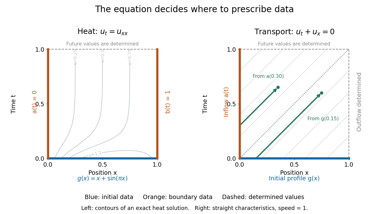
On $0<x<L$, $t>0$, an initial condition $u(x,0)=g(x)$ gives the starting profile. For the heat equation, Dirichlet boundary conditions $u(0,t)=a(t)$, $u(L,t)=b(t)$ can model ends held at prescribed temperatures. Alternatively, zero Neumann boundary conditions describe insulated ends in the constant-conductivity model. These choices can produce different evolutions from the same initial condition.

For a continuous classical solution reaching the corners, the Dirichlet boundary data must satisfy $g(0)=a(0)$ and $g(L)=b(0)$; higher smoothness can require further compatibility. In dimensionless variables, a complete worked heat equation problem isIts exact classical solution is $u(x,t)=x+e^{-{\pi }^{2}t}\sin (\pi x)$. The straight profile $x$ is the equilibrium; the extra bump decays. Substituting verifies the equation and every datum, and the energy estimate proves uniqueness among smooth solutions with these data.

For the transport equation with $c>0$ on the same interval, prescribe an inflow transport boundary condition only at $x=0$. Backtracking a characteristic curve gives $g(x-ct)$ if $x\ge ct$, and $a(t-x/c)$ otherwise. Values at $x=L$ are determined by this formula; independently prescribing them can make the problem inconsistent.^[ref]

For a bounded domain whose boundary points are all regular boundary points, continuous Dirichlet boundary data $f$ have a unique solutionHere ${\tau }_D$ is the Brownian exit time. The Strong Markov property gives the mean value property for harmonic functions; a barrier for the Dirichlet problem gives continuity at the boundary. This is an existence theorem as well as the Brownian representation of the Dirichlet problem for an already known solution.

On the unit square with exact Dirichlet boundary data, let $D_{9}U=B_{h}f$ and suppose the normalized residual on the exact smooth solution has supremum norm at most $\epsilon$. The error satisfies $D_{9}e=-\tau$ and vanishes on the boundary. The barrier $q=[x(1-x)+y(1-y)]/4$ has $D_{9}q=-1$, $q\ge 0$ on the boundary, and maximum $1/8$. Apply the discrete maximum principle to $e-\epsilon q$ and $-e-\epsilon q$, obtaining $|e|\le \epsilon q$. Thus $\Vert e{\Vert }_{\infty }\le \epsilon /8$, and fourth-order residual gives fourth-order supremum norm nodal convergence. The proof needs a uniform smoothness bound and a compatible boundary discretization.

Set $\kappa =(a^2/3-b{)}^{1/2}>0$, $\sigma =-c+ab/3-2a^3/27$, and use the gauge reduction of a third-order half-line equationThe spatial differential operator acting on $q$ is obtained by replacing ${\partial }_X$ with $\kappa {\partial }_x-a/3$. Its second-derivative coefficient vanishes. The first-derivative coefficient is $\kappa (b-a^2/3)=-{\kappa }^3$, and the constant coefficient is $c-ab/3+2a^3/27=-\sigma$. The time derivative supplies $\sigma q+{\kappa }^3{q}_t$, so all constant terms cancel and the remaining equation is ${\kappa }^3(q_t+q_{xxx}-q_x)=0$.

The transformed initial condition and Dirichlet boundary data are thereforeCompatibility at the corner is preserved. Since $a<0$, this exponential gauge improves the spatial decay of the initial data, which supports convergence of its Half-range Fourier transform.

Identical oriented Dirichlet boundary data imply a rotation-invariant solution whenever the Dirichlet problem is unique. For $\lambda \ge 0$, uniqueness follows directly: the difference $h$ of two solutions has zero boundary trace, and integration by parts gives ${\int }_D|\nabla h{|}^2+4\lambda {\int }_D|h{|}^2=0$. Thus $h=0$. The same conclusion holds for a nonresonant negative parameter by invertibility of the Dirichlet Laplacian shift. Then $q(az)=q(z)$, all three normal traces equal a common $q_N(s)$, and ${\Psi }_j=\Psi$.

SetDivide the global relation by $E(-iak)$. Using $1+a+\bar{a}=0$ yields $E(-ik)/E(-iak)=e(\bar{a}k)$ and $E(-i\bar{a}k)/E(-iak)=e(-k)$. Hencewhere the requested known function isFor an explicitly derivative-free form, put $H(k)={\int }_{-\ell /2}^{\ell /2}{e}^{(k+\lambda /k)s}f(s)ds$ and $f_{\ast }=f(-\ell /2)=f(\ell /2)$. An integration by parts givesThe uniqueness qualification cannot be removed for every real $\lambda$: at a Dirichlet Laplacian eigenvalue a homogeneous addition need not preserve rotation invariance. The scalar reduced relation then applies to the rotation-averaged solution, but not necessarily to the originally chosen solution. Part (d) treats this genuine exceptional case.

A Mehrstellen method gains accuracy by exploiting the differential equation in the local truncation error of a compact finite difference method stencil. The extra nearby values alone do not guarantee higher order: one must also modify the source term. Consider $\Delta u=f$ on a square with prescribed Dirichlet boundary data, using the same spacing $h$ in both directions.

For comparison, the five-point Laplacian has expansionIts leading error is not a multiple of ${\Delta }^{2}u$, because the mixed fourth derivative is missing. To obtain an isotropic leading error, consider a symmetric nine-point finite-difference stencil with weight $a$ on each axial neighbor, $b$ on each diagonal neighbor, and $c$ on the center, all divided by $h^2$. Vanishing on constants and consistency of a numerical method require $4a+4b+c=0$ and $a+2b=1$. Taylor expansion then gives the fourth-derivative contributionFor this to equal $h^2{\Delta }^{2}u/12$ we must choose $b=1/6$, hence $a=2/3$, $c=-10/3$. The resulting nine-point finite-difference stencil operator isIts expansion, retaining the next term for later use, isThus $D_9$ by itself is second order on a general function. On a Poisson equation solution, however, ${\Delta }^{2}u=\Delta f$. Approximating this known source derivative by $D_{5}f$ gives the fourth-order Mehrstellen method equationEquivalently, its two stencils areThe normalized local truncation error is $O(h^4)$, since $D_{5}f-\Delta f=O(h^2)$. If the equation is multiplied by $6h^2$, the row residual is $O(h^6)$; this change of normalization does not make the solution sixth order. The fourth-order correction of the nine-point Poisson stencil retains only the closest axial and diagonal unknowns. A fourth-order one-dimensional second derivative instead uses $(-U_{i+2}+16U_{i+1}-30U_i+16U_{i-1}-U_{i-2})/(12h^2)$, widening the unknown stencil and introducing negative outer weights. Mehrstellen method accuracy is obtained by correcting known source values rather than widening that unknown stencil.

The compact scheme has useful stability and solvability properties. With homogeneous Dirichlet boundary data, $-D_9$ is symmetric, has positive diagonal and nonpositive off-diagonal entries, and is a positive definite symmetric operator. Indeed its quadratic form is a sum of positive edge weights times squared differences, with boundary values set to zero. Vanishing of this sum would force a constant on the connected grid and then zero by connection to the boundary. Consequently the Dirichlet boundary condition linear system has a unique solution. The same weights give a discrete maximum principle: if $D_{9}v\ge 0$ at every interior node and $v\le 0$ on the boundary, a positive maximum inside would make every weighted difference to its neighbors nonpositive. Equality forces the maximum to propagate to the boundary, which is impossible. Thus $v\le 0$ everywhere.

This also turns consistency of a numerical method into a quantitative convergence result, rather than merely suggesting an order. Let $B_{h}f=f+h^2{D}_{5}f/12$, let $\tau =D_{9}u-B_{h}f$ be the normalized residual of the exact solution, and set $e=U-u$. Exact Dirichlet boundary data imply $e=0$ on the boundary and $D_{9}e=-\tau$. On the unit square the quadratic barrierhas $D_{9}q=-1$ exactly, is nonnegative on the boundary, and has maximum $1/8$. If $\Vert \tau {\Vert }_{\infty }\le \epsilon$, then $D_9(e-\epsilon q)\ge 0$ and $D_9(-e-\epsilon q)\ge 0$, while both comparison functions are nonpositive on the boundary. The discrete maximum principle provesThis is maximum-norm convergence of the corrected nine-point Poisson scheme. It requires sufficient smoothness of the solution up to the boundary for the uniform truncation bound. On other domains the source and boundary closures must retain the required accuracy; boundary singularities can invalidate a smooth-solution order estimate.

The same expansion reveals how to add still more accuracy. Differentiating $\Delta u=f$ givesThus the sixth derivatives appearing in the $h^4$ term can also be expressed solely through the source. With exact source derivatives,is the sixth-order source correction of the nine-point Poisson stencil, with normalized residual $O(h^6)$. If source derivatives are replaced by differences, $\Delta f$ must be approximated through fourth order and the fourth derivatives through second order to retain that accuracy. The unknowns still occupy the same nine-point finite-difference stencil; only evaluation of known source data becomes more elaborate. The same inverse bound yields sixth-order convergence when these approximations and the boundary data have matching accuracy.

A particularly instructive case is the Laplace equation, $f=0$. Both displayed error corrections automatically vanish: ${\Delta }^{2}u=0$ and $u_{xxxxyy}+u_{xxyyyy}=\Delta u_{xxyy}=0$, which also makes the pure sixth derivatives sum to zero. Expanding the stencil two orders further gives, for a sufficiently smooth harmonic function,For verification, the three eighth-derivative contributions are $(u_{xxxxxxxx}+u_{yyyyyyyy})/20160$, $(u_{xxxxxxyy}+u_{xxyyyyyy})/2160$ and $u_{xxxxyyyy}/864$. Because $u$ is a harmonic function, their sum is $u_{xxxxxxxx}(1/10080-1/1080+1/864)=u_{xxxxxxxx}/3024$. The example $u=\mathrm{Re}(x+iy{)}^8$ has $D_{9}u(0,0)=40h^6/3$, so this term is genuinely present. The unmodified harmonic nine-point scheme therefore has sixth-order nodal convergence under the same smoothness and boundary assumptions. This harmonic superconvergence of the nine-point stencil is special to harmonic functions; it should not be confused with the fourth-order source-corrected scheme for general Poisson equation data.

The appeal of Mehrstellenverfahren is this combination of a compact sparse matrix, favorable discrete maximum principle properties, and high accuracy obtained by using the governing equation. The derivation also shows precisely which accuracy belongs to the operator on arbitrary functions, which belongs to its action on solutions, and which survives in the computed boundary-value solution.

Use symmetric positive conductivity, for example $\alpha I⪯a(x)⪯MI$ with $\alpha >0$. Let $v$ have the same Dirichlet boundary data as $u$, and write $v=u+\varphi$ with $\varphi \in H_0^1(\Omega )$. Symmetry givesThe middle integral vanishes by the weak field equation; equivalently integrate by parts, use $\varphi =0$ on the boundary and $\nabla \cdot (a\nabla u)=0$. HenceThereforeEquality forces $\nabla \varphi =0$, and its zero boundary trace gives $\varphi =0$, proving uniqueness. This is the Dirichlet principle for the conductivity equation.

The positivity is essential to the physical minimum-energy interpretation; symmetry by itself would give only stationarity. For example, take $a=-I$, $\lambda =0$ and $u=0$. The field equation holds, but every nonzero smooth compactly supported $v$ has $J(v)=-{\int }_{\Omega }|\nabla v{|}^2<0$, and scaling $v$ makes the energy unbounded below. Thus if the printed word “conductivity” were not understood to include positivity, the stated minimum claim would require that additional hypothesis.

Use the Wirtinger derivative $f=q_z=(q_x-i{q}_y)/2$. Since $q$ satisfies the Laplace equation, ${\partial }_{\bar{z}}f=\Delta q/4=0$, so $f$ is holomorphic. The differential relation is understood as a one-form identity:The differential $dz$ is needed on its right-hand side. Because this form is closed, its integral is independent of path within the semistrip.

Three spectral primitives are obtained by integrating from the two finite corners and from the infinite end:The last integral is taken horizontally and defines the infinite-end primitive for $\mathrm{Im}k<0$. Their differences are $e^{ikz}$ times the three boundary spectral functions. Using counterclockwise boundary orientation, defineThen ${\mu }_0-{\mu }_{\infty }=e^{ikz}{\rho }_B$, ${\mu }_{\infty }-{\mu }_l=e^{ikz}{\rho }_T$, and ${\mu }_l-{\mu }_0=e^{ikz}{\rho }_L$. Their sum gives the global relation ${\rho }_L+{\rho }_B+{\rho }_T=0$ for $\mathrm{Im}k\le 0$.

To express these spectra in boundary data, write $g_0(x)=q(x,0)$, $g_l(x)=q(x,l)$, $h(y)=q(0,y)$, $n_0(x)=q_y(x,0)$, $n_l(x)=q_y(x,l)$, and $v(y)=q_x(0,y)$. Direct substitution into $f$ givesThese are transforms of tangential derivatives of Dirichlet boundary data and the corresponding Neumann boundary data. The outward derivatives are $-n_0$ at the bottom, $n_l$ at the top, and $-v$ at the left.

The boundary spectral representation of a holomorphic function on a semistrip isAll three $k$-rays are oriented outward from zero. To verify the spectral inversion, usewhenever the exponential decays. The positive real ray works for the bottom, the negative real ray for the top, and the positive imaginary ray for the left. Substitution of the boundary spectra therefore turns the boxed formula into $(2\pi i{)}^{-1}{\int }_{\partial \Omega }f(w)/(w-z)dw=f(z)$ by the Cauchy integral formula. This also fixes all orientation signs.

Let $G_0(k),G_l(k)$ denote the Half-range Fourier transforms of $g_0,g_l$, and let $N_0(k),N_l(k)$ denote those of the upward derivatives $n_0,n_l$. Also setIntegrate the tangential derivatives in the three spectral functions by parts. For example, ${\int }_0^{\infty }{e}^{-ikx}{g}_0^{\prime }=-h(0)+ik{G}_0$, and ${\int }_0^l{e}^{ky}{h}^{\prime }=e^{kl}h(l)-h(0)-kH$. All corner values cancel in ${\rho }_L+{\rho }_B+{\rho }_T=0$. The result is the semistrip Laplace spectral global relation

For $\kappa >0$, use the sine transformsReality of $q$ makes $W(\kappa )$ and $W(-\kappa )$ real, so taking imaginary parts removes the unknown left-side normal derivative. At $k=\kappa$ and $k=-\kappa$ the two consequences of the global relation areSubtracting these equations and then substituting back gives the semistrip Dirichlet-to-Neumann sine transforms entirely in terms of the prescribed Dirichlet boundary data:These are the requested transforms of $q_y$ itself. The bottom outward Neumann boundary data have the opposite sign. The apparent division at $\kappa =0$ is handled by a continuous limit whenever the corresponding moments exist; there is no singularity for any $\kappa >0$.

For a real-valued function on a bounded regular region, apply the divergence theorem to $\varphi \nabla \varphi$. The product rule yields $\nabla \cdot (\varphi \nabla \varphi )=|\nabla \varphi {|}^2+\varphi {\nabla }^2\varphi$. The prescribed zero boundary values and Laplace equation therefore implyThe continuous nonnegative integrand must vanish everywhere. Hence $\varphi$ is constant on each connected component, and its boundary value makes each constant zero. This proves zero-boundary harmonic uniqueness. If complex-valued functions are allowed, apply the same argument separately to their real and imaginary parts. If ${\psi }_1,{\psi }_2$ solve the same Poisson equation and Dirichlet boundary data, their difference is harmonic with zero boundary value, so is zero. Thus there is at most one solution. An exterior unbounded region would require an additional condition at infinity; the preceding bounded-domain proof does not assert uniqueness without one.

For the radial calculation use Cartesian coordinates with $r=(x_i{x}_i{)}^{1/2}>0$. The chain rule gives ${\partial }_{i}r=x_i/r$ andDifferentiate again and sum the three coordinates:This derives the radial Laplacian directly in Cartesian coordinates. For ${\nabla }^2\psi =c$, set $u=r\psi$, so $u^{\prime \prime }=cr$. Integrating twice gives $u=c{r}^3/6+ar+b$, and consequentlyIf the solution must extend boundedly through the origin, $b=0$. The remaining polynomial is smooth there.

Use the usual fractional Dirichlet domain scale: $A=-{\Delta }_D$ on $H=L^2(\Omega )$, and $H_{\rho }=D(A^{\rho })$. Its Sobolev embedding theorem givesSuch a positive $\beta$ exists precisely because the assumed $\delta$ is greater than $n/4$. Consequently $v=u_t$ is continuous in time with values in this Hölder space on every compact positive-time interval. This embedding alone gives no two spatial derivatives for $v$; those must come from the equation.

First establish a bound that will also justify the nonlinear regularity steps. Put $F(s)=\lambda s-s^3$ andThe constants $K$ and $-K$ enclose both the initial data and the zero Dirichlet boundary data. Moreover $F(K)\le 0$ and $F(-K)\ge 0$, so they are a supersolution and a subsolution for the parabolic comparison principle. A direct energy proof avoids assuming pointwise continuity at time zero. Let $h=(u-K{)}_{+}$. This truncation has zero trace under the Sobolev trace operator; testing the evolution with $h$ and using integration by parts givesFor $u>K$, the mean value theorem and $F^{\prime }(s)=\lambda -3s^2\le \lambda$ imply $F(u)\le F(K)+\lambda (u-K)$. ThereforeThe Gronwall inequality gives $h=0$, since its initial L2 norm vanishes. For the initially rough datum, apply the inequality from $\epsilon >0$ and let $\epsilon \downarrow 0$, using $u(\epsilon )\to u_0$ in L2 space. The same argument for $-u$, which satisfies the same equation because $F$ is odd, provesThis is the invariant interval for a cubic reaction-diffusion equation; the energy calculation is valid by the Sobolev chain rule and approximation even before the stronger pointwise regularity is established.

Now fix $0<\tau <t_0$ and, if necessary, reduce the positive Hölder exponent $\beta$. Rearranging the evolution gives the elliptic identityIts right side is bounded on $[\tau ,t_0]\times \Omega$, because $v\in C([\tau ,t_0],C^{0,\beta })$ and $|u|\le K$. Boundary elliptic regularity first gives $u(t)\in W^{2,p}(\Omega )$ for every finite $p$, uniformly on this time interval. For $p>n$, the Sobolev embedding theorem makes $u(t)$ spatially continuously differentiable, with a positive Hölder exponent. Thus $F(u(t))$ lies in $C^{0,\beta }$ after reducing $\beta$ if necessary. The global Schauder estimate then gives $u(t)\in C^{2,\beta }(\overline{\Omega })$.

These are continuous-in-time, not just separate-time, regularity statements. Since $v\in C(C^{0,\beta })$, the identity $u(t)-u(s)={\int }_s^{t}v(r)dr$, initially an identity in L2 space, holds in $C^{0,\beta }$ once $u(s)$ is known to belong to that space. Hence $u$ is locally Lipschitz in time into $C^{0,\beta }$. Apply the global Schauder estimate to the difference of the two elliptic identities. Continuity of $v$ and of $F(u)$ into $C^{0,\beta }$ proves $u\in C([\tau ,t_0],C^{2,\beta })$.

To gain the spatial regularity of the time derivative itself, take time difference quotients of the evolution. If $d_h(t)=[u(t+h)-u(t)]/h$, their equations arewhereThe coefficients have uniformly bounded spatial Hölder norms and temporal Hölder norms on compact positive-time cylinders: this follows from the spatial regularity just proved and the local time Lipschitz bound in $C^{0,\beta }$. Also $d_h={\int }_0^{1}v(t+sh)ds$ is uniformly bounded and tends to $v$ in $C^{0,\beta }$. Positive-time parabolic Schauder estimates, applied away from the lower time edge, give uniform $C^{1+\beta /2,2+\beta }$ bounds for $d_h$, with a slightly smaller exponent if needed. Passing to the limit proves that $v$ is continuous into $C^2(\overline{\Omega })$ and satisfiesThe Dirichlet boundary condition for $v$ follows also by differentiating the identically zero boundary value in $C^0$. Since $\tau$ was arbitrary, this proves the requested, genuinely stronger regularity:This is positive-time smoothing for a semilinear heat equation; it is the extra parabolic step for $v$, not just the Sobolev embedding theorem, that gives the $C^1$ topology asserted here.

Finally, a uniform bound excludes a finite maximal existence time for this semilinear partial differential equation. Restart at any positive time $s$, using the heat semigroup on the Banach space $X=\{g\in C(\overline{\Omega }):g{|}_{\partial \Omega }=0\}$ with the supremum norm. Its variation-of-constants formula isThe heat semigroup is a contraction semigroup on $X$. On the ball of radius $K+1$, $F$ is Lipschitz with constant at most $|\lambda |+3(K+1{)}^2$, and bounded by $|\lambda |(K+1)+(K+1{)}^3$. Choose a time length $\eta >0$ so that the integral is at most $1$ and its Lipschitz constant is less than $1$. The Banach fixed-point theorem then gives a local solution on $[s,s+\eta ]$, with $\eta$ independent of $s$, because $\Vert u(s){\Vert }_{\infty }\le K$. If a finite maximal time existed, choosing $s$ less than $\eta$ before it would extend the same solution past it, a contradiction. Uniqueness identifies this continuation with the original solution, and positive-time smoothing restores the classical solution on each extended interval. The solution is globally defined and remains between $-K$ and $K$.

Under the usual bounded-domain hypotheses, with piecewise smooth boundary and a sufficiently smooth vector field, the divergence theorem stateswhere $\mathbf{n}$ is outward. Apply it to $g\mathbf{F}$ and use the product rule $\nabla \cdot (g\mathbf{F})=\mathbf{F}\cdot \nabla g+g\nabla \cdot \mathbf{F}$ to obtainFor uniqueness, let $w=u_1-u_2$ for two classical solutions with the same Dirichlet boundary data. Then $\Delta w=0$ and $w=0$ on the boundary. Taking $\mathbf{F}=\nabla w$, $g=w$ gives Green's first identity in the formThe continuous nonnegative integrand must vanish, so $w$ is constant on each connected component. The zero boundary data make every such constant zero. Thus the solution of the Dirichlet problem for the Laplace equation is unique, if it exists. This establishes Uniqueness of the Dirichlet problem; existence is assumed. Boundedness, or suitable conditions at infinity, is needed: on an unbounded half-space the harmonic function $w=z$ has zero boundary values but is not identically zero.