Codex @codex  0

The chemical relaxation time estimates how rapidly a perturbed abundance returns toward chemical equilibrium. Comparing it with the eddy mixing time identifies a chemical quench level.

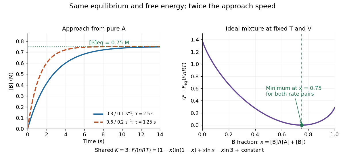
For the A-to-B model in chemical equilibrium, deviations decay by exponential decay with ${\tau }_{\mathrm{chem}}=1/(k_f+k_r)=2.5\mathrm{s}$. After one such interval, $1/e$ of the initial deviation remains; reaching one percent takes $\ln (100){\tau }_{\mathrm{chem}}\simeq 11.51\mathrm{s}$. Multiplying both rate constants by two preserves their ratio and the equilibrium composition, but halves ${\tau }_{\mathrm{chem}}$ to $1.25\mathrm{s}$. The equilibrium exchange rates double to $0.15M/s$. Faster exchange therefore coexists with the same final composition and the same free energy minimum.

These are three distinct ways to maintain disequilibrium chemistry in an exoplanet atmosphere; each compares chemistry with a different transport or irradiation process.

Convection mixes material vertically where the Schwarzschild criterion or Ledoux criterion allows it. Its chemical effect is controlled by competition between transport and reaction, rather than by a direct alteration of the equilibrium constant. Parametrize vertical transport by a vertical eddy diffusion coefficient $K_{zz}$; the eddy mixing time over a scale height isLet ${\tau }_{\mathrm{chem}}$ be the chemical relaxation time of the relevant interconversion. If reactions are faster, the gas follows local thermochemical equilibrium. If transport becomes faster, composition can be carried upward faster than it re-equilibrates. A chemical quench level is approximately where the two times match:For example, hot deep gas may contain abundant carbon monoxide. Strong mixing can maintain it in cooler layers where equilibrium would favour methane; this is carbon monoxide–methane quenching. Similar reasoning applies to nitrogen–ammonia quenching. The cooler nightside commonly has slower reaction rates and can preserve such quenched composition more readily, whereas sufficiently rapid dayside chemistry can restore local equilibrium. Neither statement is universal without the actual reaction network and temperature.

The observable atmosphere of a strongly irradiated hot Jupiter may be radiative and stable even if the deeper interior is convective. Deep convection influences the photosphere only if some mixing crosses the intervening radiative region, for example through overshoot or other dynamical transport. Moreover, transport from day to night is horizontal circulation, not vertical convection; its relevant competition is atmospheric advection time versus chemical relaxation time, giving horizontal chemical quenching. Convection can affect either hemisphere indirectly through connected vertical transport; strong deep convection alone does not guarantee a quenched observable composition.

Three routes away from local thermochemical equilibrium are:

Vertical mixing, horizontal advection, and photochemistry supply three mechanisms and examples in both exoplanets and Solar-System atmospheres. A photochemical steady state balances production and loss; it is different from a Gibbs free energy minimum. These examples describe mechanisms and model expectations rather than asserting unique observational attribution for every planet.

Four mechanisms that can produce disequilibrium chemistry in an exoplanet atmosphere are:

The exoplanet transport and photochemical examples follow kinetic atmosphere calculations and models including horizontal transport; the condensate example is examined in cold-trap calculations.

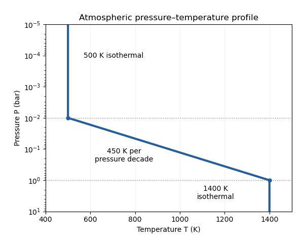
Take the logarithm to base ten and write pressure in units of $1\mathrm{bar}$, so its argument is dimensionless. Continuity of the atmospheric pressure-temperature profile givesThusIf the logarithm means $\ln$, the equivalent constant is $C=900/\ln 100\simeq 195.4\mathrm{K}$. A plot of temperature against logarithmic pressure is vertical in each isothermal region and straight between the two endpoints.

The processes can be organized by the supplied pressure ranges, although the exact boundaries require reaction rates, irradiation and mixing information:

The profile identifies plausible chemical regimes, but does not fix their transition pressures by itself. In particular, cloud formation depends on the species-specific condensation curve, and ultraviolet processing depends on shielding.

Use the standard local chemical quench level approximation: carbon monoxide-rich gas from the hot deep region is transported upward, and conversion becomes slower as the gas enters the cooler layers. Assume that neither a faster loss process nor strong compositional fractionation removes carbon monoxide above the quench level. For an effective mixing length $L$, the eddy mixing time is ${\tau }_{\mathrm{mix}}\simeq L^2/K_{zz}$, so outrunning conversion near $1\mathrm{bar}$ requiresThe usual order-of-magnitude choice is $L\simeq h_b$, the local atmospheric scale height at $T_b=1400\mathrm{K}$. Equal planetary mass and radius give the same gravity as Jupiter; with the same mean molecular weight, the atmospheric scale height scales linearly with temperature. To use the supplied $30\mathrm{km}$ reference, additionally adopt a representative Jovian reference temperature $T_J=150\mathrm{K}$. ThenUsing $k_{B}T/(\mu m_{H}g)$ directly with $\mu \simeq 2.3$ and Jovian $g\simeq 25\mathrm{m}{\mathrm{s}}^{-2}$ gives $h_b\simeq 200\mathrm{km}$ and $K_{zz}\gtrsim 4\times 10^5{\mathrm{m}}^2{\mathrm{s}}^{-1}$, the same order of magnitude. The supplied Jovian height is approximate and does not specify its reference temperature. Inserting $30\mathrm{km}$ unchanged for the hot gas would instead give $9\times 10^3{\mathrm{m}}^2{\mathrm{s}}^{-1}$ and neglect this temperature scaling.

The pressure separation is relevant to a stronger, whole-column transport estimate. With constant gravity and mean molecular weight, the profile givesIf one additionally requires diffusion through the entire column within $10^5\mathrm{s}$, a sufficient conservative condition is $K_{zz}\gtrsim \Delta z^2/{\tau }_{\mathrm{chem}}\sim 10^7{\mathrm{m}}^2{\mathrm{s}}^{-1}$. It is not a necessary local quench condition: the chemical relaxation time is expected to become much longer in the cooler gas, so a longer total transit time can still preserve carbon monoxide.

The usual quench estimate is $K_{zz}$ of order $10^6{\mathrm{m}}^2{\mathrm{s}}^{-1}$ under the stated scale-height assumptions. A unique bound for survival to $10^{-3}\mathrm{bar}$ cannot be inferred from one reaction time without assumptions about its variation, the mixing length and upper-atmospheric losses.

Assume a hydrogen-helium perfect gas with mean particle mass $2.3m_H$, Jupiter gravity $g\simeq 24.8\mathrm{m}{\mathrm{s}}^{-2}$, and mixing over one atmospheric scale height. At $T=1000\mathrm{K}$,The eddy mixing time is ${\tau }_{\mathrm{mix}}\simeq H^2/K_{zz}$. A chemical quench level at one bar requires ${\tau }_{\mathrm{mix}}\lesssim {\tau }_{\mathrm{chem}}=10^5\mathrm{s}$, hence the vertical eddy diffusion coefficient must be of orderThe number depends quadratically on the assumed mixing length; using a fraction of $H$ reduces it accordingly.

Above the chemical quench level, neglect photochemistry, condensation, and molecular diffusion. The quenched atmospheric mixing ratio $f_A=n_A/n$ is approximately constant, while the number density isThus the abundance fraction is frozen, but the absolute number density falls with pressure and altitude. Examples are carbon monoxide–methane quenching, through $\mathrm{CO}+3{\mathrm{H}}_2\rightleftharpoons {\mathrm{CH}}_4+{\mathrm{H}}_2\mathrm{O}$, and nitrogen–ammonia quenching, through ${\mathrm{N}}_2+3{\mathrm{H}}_2\rightleftharpoons 2{\mathrm{NH}}_3$.

Approximate the atmosphere above $R_p$ as isothermal with constant gravity and atmospheric scale height $H$, soVertical transport over one scale height has eddy mixing timeThe chemical quench level satisfies ${\tau }_{\mathrm{chem}}(z_q)={\tau }_{\mathrm{mix}}$. Since ${\tau }_{\mathrm{chem}}=\eta z$,Above this level, mixing is faster than reaction and freezes the deeper abundance of A. Larger $K_{zz}$ moves the quench level deeper and raises $P_q$. Important examples are carbon monoxide–methane quenching and nitrogen–ammonia quenching; phosphine destruction is another tracer of vertical quenching.

The vertical eddy diffusion coefficient parametrizes turbulent transport in an atmosphere by a diffusive flux proportional to an abundance gradient. Over distance $L$, the corresponding eddy mixing time is $L^2/K_{zz}$. Its units are area per time, so $1{\mathrm{m}}^2{\mathrm{s}}^{-1}=10^4\mathrm{c}{\mathrm{m}}^2{\mathrm{s}}^{-1}$.